CASP10-BCL::Fold efficiently samples topologies of large proteins

Abstract

During CASP10 in summer 2012, we tested BCL::Fold for prediction of free modeling (FM) and template-based modeling (TBM) targets. BCL::Fold assembles the tertiary structure of a protein from predicted secondary structure elements (SSEs) omitting more flexible loop regions early on. This approach enables the sampling of conformational space for larger proteins with more complex topologies. In preparation of CASP11, we analyzed the quality of CASP10 models throughout the prediction pipeline to understand BCL::Fold’s ability to sample the native topology, identify native-like models by scoring and/or clustering approaches, and our ability to add loop regions and side chains to initial SSE-only models. The standout observation is that BCL::Fold sampled topologies with a GDT_TS score > 33% for 12 of 18 and with a topology score > 0.8 for 11 of 18 test cases de novo. Despite the sampling success of BCL::Fold, significant challenges still exist in clustering and loop generation stages of the pipeline. The clustering approach employed for model selection often failed to identify the most native-like assembly of SSEs for further refinement and submission. It was also observed that for some β-strand proteins model refinement failed as β-strands were not properly aligned to form hydrogen bonds removing otherwise accurate models from the pool. Further, BCL::Fold samples frequently non-natural topologies that require loop regions to pass through the center of the protein.

INTRODUCTION

Experimental structures in the protein data bank (PDB) are biased toward small soluble proteins

The tertiary structure of a protein provides essential insights to its biological function in living organisms. Accordingly, experimental methods are applied to ascertain protein structure including X-ray crystallography and nuclear magnetic resonance (NMR) spectroscopy. Currently, the PDB contains more than 89,258 proteins (December 2013) of which 79,585 (89%) were elucidated by X-ray crystallography, 8971 (10%) by NMR, and the remainder by other technologies.¹ Despite these efforts, the structures represented in the PDB are biased; 87,004 of the proteins in the PDB are soluble while only 2254 (2.5%) of the proteins represent membrane proteins.¹ Further, the size distribution of proteins in the PDB is biased toward small proteins omitting many large macromolecular assemblies greater than 500,000 Da (2.0%).^1–3 This bias is due to the limitations of experimental methods for structure determination. Membrane proteins are underrepresented in the PDB because they are too large for NMR and their embedding in the two-dimensional membrane complicates formation of three-dimensional crystals required in X-ray crystallography.⁴ For membrane proteins up to ~1000 folds remain to be determined.^5,6 Large macromolecular assemblies are also underrepresented in the PDB because its protomers do not fold in isolation, they are difficult to crystallize, and they are too large for NMR spectroscopic methods.⁷ Thus, for many biologically relevant proteins only limited experimental data can be collected with a combination of experimental techniques such as solid state NMR, cryo-electron microscopy, electron paramagnetic resonance, mass spectrometry, and small angle X-ray scattering. On their own, these datasets are insufficient for atomic-detail structure determination. One major justification to develop de novo protein structure prediction algorithms is to complement such limited experimental datasets.

De novo protein structure prediction needs a reduced search space

The cornerstone of de novo protein structure prediction methods is based on the assumption that (most) folded proteins exist in their lowest energy conformation.⁸ Protein folding becomes an energy minimization process that depends on interaction of amino acids with the environment and other amino acids in the sequence. Finding the global minimum of the energy function on the energy landscape is challenging for several reasons including that the energy landscape contains many local minima. Currently, no universal method of identifying the global minimum of the energy function exists.⁹ In practice, the conformational space of a protein is also far too large to be comprehensively searched with a highly accurate and therefore slow to compute energy function. Therefore, the conformational space is reduced by working with simplified protein representations, at least in the initial folding simulation. In effect, this reduces the resolution of the energy function which allows a more rapid calculation but decreases its accuracy to the point where the global energy minimum cannot be unambiguously detected and several local energy minima need to be considered.

Competing de novo structure prediction software reduces the search space similarly. Rosetta addresses the sampling challenge by assembling protein models from three and nine residue peptide fragments.^10–12 These fragments are determined from peptides of similar sequence and secondary structure extracted from other proteins in the PDB. For proteins smaller than 80 residues Rosetta was able to predict atomic detail models in the absence of any experimental restraints for about 30% of the test cases.¹³ For larger proteins up to around 150–180 residues Rosetta samples the correct topology about 50% of the time.^13–15 Generally, Rosetta tends to perform better for α-helical proteins which is related to their reduced fold complexity. The complexity of a fold can be measured by contact order (CO) which is defined as the average sequence separation of residues in contact, that is, residues whose C_β atoms are <8 Å apart.^16,17 As the complexity of protein topology increases (high CO) the accuracy of the Rosetta prediction decreases.^16,18

I-Tasser threads the target sequences through a library of PDB structures with a pair-wise sequence identity cut-off of 70% to search for plausible protein folds. Rather than using a fixed set of three and nine residue peptide fragments, I-Tasser uses fragments of variable size that are identified by threading.^19–21 The fragments are used to reassemble full-length models while the loop regions between fragments being constructed de novo. Critical to the success of I-Tasser is the identification of a suitable templates to create the peptide fragments—a Pearson correlation coefficient of 0.89 for RMSD and 0.95 for TM-score.²¹ Generally, I-Tasser samples the correct topology about a third of the time for proteins up to 155 residues long with RMSD < 6.5 Å.²¹ I-Tasser shares the most critical limitation with Rosetta, the ready formation of long-range interactions between residues.

BCL::Fold was designed to overcome size and complexity limitations in de novo protein structure prediction methods

BCL::Fold is a de novo protein structure prediction algorithm based on the placement of disconnected secondary structure elements (SSEs) in three-dimensional space as previously published.^6,22,23 This algorithm was developed to test the hypothesis that for many proteins the core responsible for thermodynamic stability is largely formed by SSEs. In this case, likely protein topologies could be detected from SSE-only models. Thereby, the size and CO restrictions in protein structure prediction can be overcome by assembling disconnected, rather rigid SSEs, reducing the search space substantially and allowing the ready formation of nonlocal contacts.²² A coarse grained knowledge based energy function identifies native-like SSE arrangements using a Monte Carlo simulated annealing sampling algorithm with Metropolis criterion.^6,22,23 In contrast to I-Tasser or Rosetta, this algorithm is truly de novo as no fragments from the PDB are used. Loop regions between SSEs and side chains atoms are added to the model in subsequent steps using for example Rosetta.^24–26

BCL::Fold uses a consensus of secondary structure prediction technologies to identify SSEs

Critical to the success of the BCL::Fold algorithm is the correct prediction of SSEs: α-helices, β-strands, coil regions, and trans-membrane spans from sequence. These predictions are obtained from a consensus prediction from PHD,^27,28 PsiPred,^29,30 and Jufo9D^31–33 for soluble proteins. In addition to these methods we used Octopus^34,35 and Jufo9D³¹ for the trans-membrane span region of membrane proteins. The consensus prediction is used to build a pool of SSEs, which is input for protein folding.

A Monte Carlo Metropolis sampling algorithm positions SSEs in space

Protein models are assembled using a Monte Carlo sampling algorithm. Each iteration of the algorithm consists of a randomly selected modification to the current model. Modifications include the addition of an SSE from the SSE pool to the model; the removal of an SSE from the model; translational and rotational transformations of SSEs in the model; swapping of two SSEs; modifications of groups of SSEs (domains) consist of translating the domain; flipping; and shuffling the different SSEs.

After each modification, the model is evaluated by a knowledge based scoring function.²³ This coarse grained scoring function is designed to evaluate the arrangement of SSEs in Euclidean space. It is a weighted sum of scoring terms that represent different aspects of SSEs of protein structures as observed in experimental structures like the preferred environment of amino acid types (buried or solvent exposed); the radius of gyration; an SSE packing and a strand pairing potential; a loop length potential; clash terms for amino acids and SSEs; and a loop closure penalty. The loop closure penalty limits the Euclidean distance between two consecutive SSEs to the maximum length a stretched out amino acid chain can bridge and applies a steep penalty for longer loop distances.

The evaluation with the Metropolis criterion results in one of four possible outcomes: (1) improved and accepted, if the calculated energy score is lower than the energy of the previous model; (2) accepted by the Metropolis criterion with a function taking the energy difference and the simulated temperature into account; (3) rejected if the score is higher than the previous model and rejected by the Metropolis criterion; (4) skipped, if the modification is not applicable to the model, for example swapping SSEs if the model contains only a single SSE. The probability of a step being accepted with higher energy is based on the temperature used by the Metropolis criterion. BCL::Fold adjusts the temperature to achieve a ratio of accepted steps that reduces from 50 to 20% in the course of the simulation.

All scoring terms (except for the clash terms and the loop closure penalty) are statistically derived using Bayes’ theorem from a divergent high resolution subset of the PDB generated by the PISCES server with a maximum sequence identity of 25%^36,37 and then energies were approximated using the inverse Boltzmann relation.

The algorithm will continue generating modified models and evaluating them until a maximum number of 2000 steps was completed or no improvement in the score was found for 400 consecutive steps; this constitutes one folding stage. The folding process of one model has five assembly stages and one refinement stage, which employ a decreasing number of modifications for large scale perturbations (for example, swapping SSEs) and an increasing amount of small scale perturbations (for example, bending an SSE). The lowest energy model within the trajectory will be saved as resulting model for this run.

The CASP10 experiment: a critical tool for development of techniques for protein structure prediction

To evaluate the accuracy of BCL::Fold in de novo protein structure prediction, we participated in the Critical Assessment of protein Structure Prediction (CASP10) experiment, which is held every two years.^38,39 The double-blind experiment tests protein structure prediction methods objectively because the experimentally determined structure is withheld from predictors, organizers and the assessors until the experiment is finished. After protein predictions have been made, the experimentally determined structures are revealed and the results are assessed. CASP10 contained the following categories: (1) Tertiary structure prediction, which can be classified as: (a) Template Based Modeling (TBM): starting from a homologous protein template in the PDB. (b) Free Modeling (FM): no homologous template exists in the PDB; (2) Tertiary structure prediction with limited experimental information, for example, amino acids in contact⁴⁰; (3) Residue-residue contact prediction⁴¹; (4) Model refinement⁴²; (5) Identification of disordered regions; (6) Function prediction; (7) Quality assessment.⁴³

To maximally leverage CASP10 for testing BCL::Fold we assume all CASP10 targets to be FM targets

For some targets, templates can be found, that is, proteins with similar sequence and known structure that can guide the prediction. Based on if templates can be found and how similar the template structure is to the target structure, measured by the Global Distance Test/Total Score (GDT_TS),⁴⁴ prediction for CASP10 targets is categorized as easy or hard TBM (easy if the maximal GDT_TS ≥ 50, hard if the maximal GDT_TS < 50), FM or a combination of both (TBM/FM). The GDT_TS could obviously only be employed after the target structures were available; in the prediction process other measures like sequence similarity to proteins in the PDB were used to classify targets. To maximize the assessment of the BCL::Fold de novo protein structure prediction algorithm in CASP10 we treated all targets as FM targets, that is, no homologous template from the PDB was used at any point as input into the BCL::Fold prediction algorithm.

MATERIAL AND METHODS

Secondary structure and transmembrane span prediction

In the first step, the secondary structure is predicted for soluble proteins using Jufo9D,^31–33 PsiPred,^29,30 and ProfPHD.^27,28 For membrane proteins Jufo9D³¹ and Octopus^34,35 are used to detect secondary structure and transmembrane spans. From the predicted secondary structures, a pool is created for use by BCL::Fold as described before.²² The pool is manually examined to ensure a complete as possible set of SSEs.

Fold recognition and domain identification

Fold recognition methods combined in bioinfo.pl were used to see if the target sequence contains multiple domains,⁴⁵ and if proteins of those folds have been experimentally determined. If the fold recognition result indicated that the target has multiple domains, the SSE pool is split up into sub pools according to the domain boundaries.

BCL::Fold folding simulation

BCL::Fold is run next to produce 12,000 models for each domain of one target. Depending on the target, the soluble or membrane protocol is employed. For each model, a completeness estimate is calculated as fraction of the sum of the sequence lengths of all SSEs in the models to the total sequence length of the target. Models that are 2% less complete than the average model produced are removed.

Clustering to identify topologies that reside in wide energy funnels

After filtering the 12,000 models per target by completeness score, models were selected by three criteria for further refinement. The first method for selection was clustering by average RMSD linkage between models where the clusters ideally only contain models with the same fold. Cluster sizes varied with the largest clusters having a few hundred models and the smallest clusters containing a few or even a single model. Cluster radii leafs were between 0 and 18 Å with most at 10 Å. The RMSD cutoff was manually adjusted based on protein size and model similarity. Up to five models from each cluster were selected for further refinement. The second method for selection was ranking by the BCL scoring function. All filtered models were sorted by BCL sum score and the lowest scoring models were selected. The third method was only used if we successfully identified a template model of the target protein and models were pooled into a separate set. In this case, the RMSD between the template and BCL generated models were computed. The models with the highest similarity (lowest RMSD) were selected for further refinement. Furthermore, in some cases the selected models were visually inspected in PyMOL to evaluate sequence length and Euclidean distances for later loop reconstruction. In this step, some models were removed from further processing if loops went through the center of the protein core (Table I).

Table I.

Clustering Statistics of CASP10 Targets folded by BCL::Fold.

Target	Folded models	After filtering	Top cluster	Top scoring	Top homology
T0644	9980	4485	2	0	0
T0649	10,000	5135	3	5	0
T0655	9980	4335	1	3	2
T0663	12,000	6495	3	2	3
T0666	12,000	5979	3	3	0
T0676	12,000	6341	3	0	1
T0678	12,000	6371	5	1	2
T0682	12,000	5554	0	3	4
T0684	12,000	5884	16	0	1
T0686	12,000	6230	2	1	0
T0691	12,000	6083	4	1	2
T0700	12,000	6605	1	2	3
T0704	12,000	5932	1	3	1
T0720	12,000	6345	2	2	1
T0722	12,000	8747	1	2	1
T0724	11,999	5886	3	1	0
T0743	12,000	6374	2	2	4
T0745	12,000	6108	2	2	0

Combining domains into complete models

If the target consisted of multiple domains, models of all possible combinations of domains are created either by arranging the domains in space close to each other or, if possible, by aligning the domain models to a template. The domains do not have to be connected by creating a loop at this point, because all models consist of only SSEs and loops will be built in the next step.

Loop construction using cyclic coordinate decent

Adding loops is a two-step process of inserting the missing amino acids in a model and creating coordinates for them by CCD. Once SSEs have been placed, loop regions between SSEs must be built. Creating loops is a two-step process of inserting the missing amino acids in a model and creating coordinates for them. This is accomplished by adding loop residues using (1) knowledge based potentials, (2) likely phi and psi backbone angles, and (3) cyclic coordinate descent (CCD). The first step is to dynamically add missing residues in the loop region. Residues are added with initial phi and psi angles derived from a probability distribution of experimentally observed angles. They are then perturbed and scored using a knowledge based potential for native like angles. This potential has scoring terms that penalize clashes between atoms using van der Waals radii, compare the sequence length with the Euclidean distance, measure the gap between adjacent SSEs, incorporate angles derived from Ramachandran plots, and score the likelihood that the distance between the SSEs can be closed by a loop. Once the initial residue coordinates of the loop region have been placed, CCD⁴⁶ is used to minimize the distance between a freely moving and fixed set of coordinates to close a loop. In this second step, an additional penalty term is added to the scoring function that scores how close the residue at the loop end is to the pseudo residue at the N terminus of the target SSE. Between 200 and 8400 loop models were build depending on model size and complexity to achieve a sufficiently low BCL sum score that is, in a similar score range than the nonloop start model. Models with loops difficult to close were either modified to allow an easier loop closure by shortening the SSEs adjacent to the loop or they were removed from further modeling. The best scoring loop models according to the BCL sum score were further processed.

Addition of side chains and model relaxation

One of two methods was used: either side chains were added with a relax step in which the relative position of the amino acids were restrained, or, if the first method fails because of misaligned β-strands, by adding and repacking side chains. Between 10 and 200 side-chain models were built to obtain an optimal overall Rosetta score.

Model selection for submission

From the lowest scoring side chain models for each loop model, the ones deemed most native-like by visual inspection were selected for CASP10 submission. If a template model and a similar BCL model were found before, it was selected as the fifth submitted model.

Topology score to evaluate protein models

To evaluate if BCL::Fold can sample the folding space required for our target proteins, we introduce a new measure that focuses on SSE contacts instead of comparing atom positions like RMSD100⁴⁷ or GDT.⁴⁴ This new measure computes the similarity of a model to a native protein by calculating the fraction of SSE contacts of the native that are present in a given model and the total number of SSE contacts of the native (true positive rate, sensitivity). An SSE contact is assumed if the distance of the central axis of two SSEs is less than a certain threshold. An SSE can be represented by its central axis for the purpose of the distance calculation, because all SSEs in a BCL model are idealized. The threshold below which two SSEs are assumed in contact depends on the type of SSE contact (helix-helix: 16 Å; helix-sheet: 16 Å; strandstrand: 5.5 Å; sheet-sheet: 14 Å) and was derived from native protein structures from the PDB. These thresholds were chosen to be large to be as inclusive as possible. The strength of the interaction is represented by line thickness of the connecting lines (Fig. 4).

Figure 4.

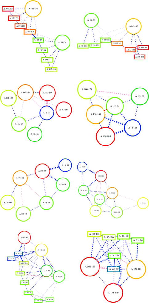
Visualization of the topologies for the native and the best scoring model according to the topology score for selected target showing both successful (T0663, T0666, and T0682 in order from the top down with topology scores of 0.81, 0.82, and 1.00 for the respective best scoring model) and unsuccessful cases (T0655 at the bottom with a topology score of 0.44). [Color figure can be viewed in the online issue, which is available at wileyonlinelibrary.com.]

RESULTS

Eighteen targets included in this analysis

During CASP10 a total of 53 targets were released for human predictors. Eighteen of these had at least one domain in the FM category. To focus our efforts we excluded proteins that were very small (<50 residues) or very large (>400 residues). Further, for some targets calculations did not finish in time for submission. For 21 targets models were submitted, five of them in the FM category. For two targets files were corrupted on our server, for one target no experimental structure has been released. This leaves 18 targets, three in the FM category, for analysis (Table II). Accordingly, treatment of the TBM targets as FM targets substantially increased the number of proteins that could be included in the study beyond the small number of FM targets. One consequence of this procedure is that BCL::Fold will not rank among top methods for the TBM section, as we do not expect BCL::Fold to predict protein structure more accurately than comparative modeling.

Table II.

Statistics on 18 CASP10 Targets Predicted with BCL::Fold.

Target	PDB ID	Length	NCO	Category	Oligomeric state	Domains	α-Helices	TM α-helices	β-strands
T0644	4FR9	166	22.1	TBM-easy	Monomer	1	2	0	8
T0649	4F54	210	58.9	TBM-hard	Monomer	1	4	0	9
T0655	2LUZ	182	44.2	TBM-easy	Monomer	3	4	0	8
T0663	4EXR	205	28.4	FM	Monomer	2	2	0	8
T0666	3UX4	195	64.9	FM	Trimer	1	6	6	0
T0676	4E6F	204	45.2	TBM-hard	Dimer	1	4	0	7
T0678	4EPZ	161	30.5	TM-hard	Monomer	1	7	0	0
T0682	4JQ6	235	63.5	TMB-easy	Trimer	1	7	7	0
T0684	4GL6	270	36.9	FM	Dimer	2	8	0	8
T0686	4HQO	259	55.7	TMB-easy	Dimer	3	4	0	5
T0691	4GZV	163	25.7	TMB-easy	Monomer	3	0	0	8
T0700	4HFX	86	18.0	TMB-easy	Tetramer	2	3	0	0
T0704	4HG2	254	55.4	TMB-easy	Dimer	3	9	0	8
T0720	4IC1	202	47.5	TMB-easy	Monomer	1	7	0	6
T0722	4FLA	152	44.1	Cancelled	Tetramer	Cancelled	4	0	0
T0724	4FMR	265	42.6	TMB-easy	Tetramer	2	4, 5	0	16
T0743	4HYZ	149	36.9	TMB-easy	Monomer	1	4	0	5
T0745	4FMW	185	49.4	Cancelled	Dimer	Cancelled	6	0	6

An automated pipeline with minimal human intervention was setup

Here we give an overview of the overall protocol (Fig. 1). A detailed description of the individual steps is given in the methods section. The folding pipeline starts with the downloaded target sequence from CASP10 Prediction center. In the first step, secondary structure and transmembrane spanning regions are predicted and stored in a “pool” using the consensus SSE prediction results. The SSE pool is manually examined to ensure that weakly predicted SSEs are available. Domain boundaries were identified with bioinfo.pl - a consensus fold recognition Meta server.⁴⁵ At this stage of folding, templates were identified for TBM targets and comparative models were constructed using the Modeler^24–26 link of the bioinfo.pl server. The homology model was saved for later analysis or prioritization of the de novo folded models. It was not used to bias the folding simulation. If the fold recognition result from bioinfo.pl indicated that the target consisted of multiple domains, the SSE pool was split into subpools according to the domain boundaries. Next, each domain was folded 12,000 times with BCL::Fold. Resulting models were filtered for completeness before entering the clustering protocol. The completeness estimate is the total number of residues in SSEs divided by the total number of residues in the protein model. The filtering cutoff is the average of all the completeness estimates reduced by 0.01. After filtering, cluster centers of the 10 to 20 largest clusters were selected for further processing. In addition, we included the five best scoring models measured by the BCL sum score. If templates were identified, best-scoring models that were similar to the template by Mammoth z-score⁴⁸ were retained in a separate pool of models. If the target was split into multiple domains, these were recombined at this stage. The backbone of the resulting models was completed using a Cyclic Coordinate Decent (CCD)⁴⁶ loop closure algorithm within the BCL. Afterwards, side chain coordinates were constructed and the model was relaxed using Rosetta. From the resulting set of up to 200 models, five were chosen for submission by Rosetta energy. If a template has been identified, the fifth model submitted was chosen from the second pool as the one most similar to the template, to assess BCL::Fold’s sampling capability independent from scoring.

Figure 1.

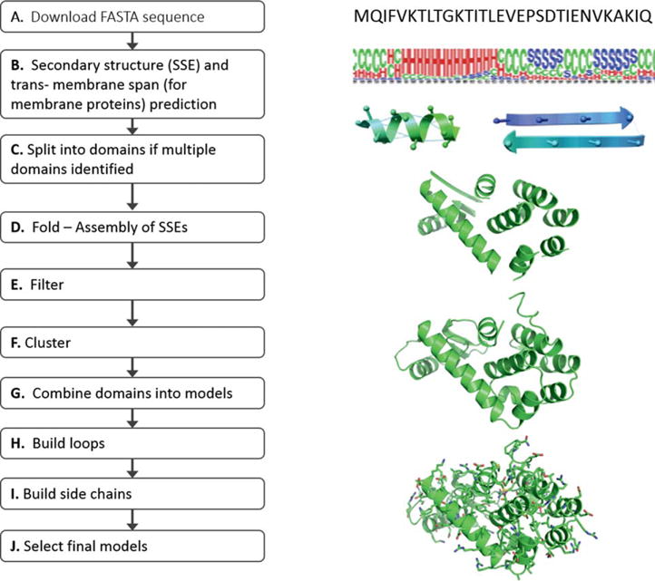
CASP10 Pipeline. Obtain target sequence from CASP10 prediction center (A); Perform SSE prediction (B); Split multimeric proteins into individual domains (C); Assemble SSEs in Folding algorithm, analyze fold models, compare generated models with native secondary structure, evaluate loop closure potential and beta sheet register shift (D); Filter erroneous models from further analysis (E); Cluster predicted folds and analyze cluster centers (F); Combine domains if previously split (G); Reconstruct loop regions and analyze models (H); Build side chains with Rosetta or other high resolution refinement software (I); Select final models and analyze final model selection (J). [Color figure can be viewed in the online issue, which is available at wileyonlinelibrary.com.]

Accuracy of secondary structure and transmembrane span prediction

Table III depicts Q3 accuracies (a measure of the accuracy for predicting per residue secondary structure), the percentage of native secondary structures correctly predicted and the average shifts for the SSE pools of the 18 CASP10 protein targets. The shift values are the sum of the deviations in the first and last residues of the predicted SSEs when compared with native SSEs. The overall average percentage of native secondary structures correctly predicted (% found) using PHD,^27,28 PSIPRED,^29,30 and JUFO9D^31–33 was 91.8%. In the original benchmark of BCL, the overall average % found was 96.6%.²² We achieve the highest overall accuracy by combining multiple secondary structure prediction methods to create the SSE pool, rather than relying on a single secondary structure prediction method. For example, the % found values for PHD, PSIPRED, and JUFO9D are 78.9, 91.0, and 91.4%, respectively. In the original BCL benchmark, these values for PSIPRED and JUFO are 96.1 and 90.3%, respectively. This indicates that the secondary structure prediction is more challenging for the CASP10 targets than the original BCL benchmark. In addition, during a folding run, BCL::Fold can merge, grow, or shrink SSEs based on the predicted probabilities.

Table III.

Secondary Structure Pool Statistics for CASP10 Targets

		PHD			PSIPRED			JUFO9D			Combined
Target	PDB ID	Q3	% Found	Shift	Q3	% Found	Shift	Q3	% Found	Shift	% Found	Shift
T0644	4FR9	68.7	80.0	1.8	80.1	100.0	1.1	77.7	100.0	1.5	100.0	0.9
T0649	4F54	63.8	53.8	6.0	71.9	69.2	5.2	65.2	76.9	5.3	61.5	2.9
T0655	2LUZ	54.9	75.0	5.4	76.4	91.7	3.7	70.9	91.7	4.4	66.7	3.5
T0663	4EXR	54.1	80.0	2.9	80.5	100.0	1.5	69.3	100.0	1.8	90.0	0.9
T0666	3UX4	50.3	57.1	9.5	74.9	85.7	8.3	81.0	85.7	7.0	85.7	4.8
T0676	4E6F	66.7	80.0	8.9	77.9	90.0	1.9	57.4	90.0	7.3	90.0	1.3
T0678	4EPZ	72.0	85.7	11.7	83.2	100.0	2.7	78.9	100.0	3.4	100.0	1.3
T0682	4JQ6	62.6	100.0	14.1	71.1	100.0	10.6	79.1	100.0	11.6	100.0	4.0
T0684	4GL6	72.2	81.3	3.4	73.7	87.5	2.9	67.8	75.0	3.2	100.0	1.9
T0686	4HQO	64.1	72.2	5.0	74.5	66.7	2.8	67.6	88.9	4.3	94.4	3.4
T0691	4GZV	47.9	75.0	4.7	69.9	100.0	3.6	59.5	100.0	4.8	100.0	3.3
T0700	4HFX	74.4	100.0	5.0	75.6	100.0	4.3	72.1	100.0	3.3	100.0	2.7
T0704	4HG2	63.0	58.8	3.1	74.8	88.2	3.3	72.0	88.2	2.8	94.1	2.1
T0720	4IC1	70.3	84.6	5.5	84.2	92.3	3.6	79.2	92.3	3.8	92.3	3.3
T0722	4FLA	87.5	100.0	30.0	89.5	100.0	9.0	80.3	100.0	16.5	100.0	7.0
T0724	4FMR	71.3	84.2	2.9	86.0	89.5	1.8	78.5	94.7	1.7	89.5	1.2
T0743	4HYZ	72.5	77.8	3.7	77.2	77.8	2.7	67.8	77.8	6.6	88.9	1.8
T0745	4FMW	65.9	75.0	2.8	77.3	100.0	1.9	67.6	83.3	2.9	100.0	1.8
Average		65.7	78.9	7.0	77.7	91.0	3.9	71.8	91.4	5.1	91.8	2.7
Std Dev		9.6	13.4	6.6	5.3	10.7	2.7	7.2	8.8	3.8	11.3	1.6

Quality of CASP10 FM models submitted by other research groups

There were 20 FM targets in CASP10. For all participating methods the average GDT_TS score ranged from 7.0 to 36.0% with a mean GDT_TS score of 21.7% and a standard deviation of 7.2%. The maximum GDT_TS score ranged from 16.5 to 44.0% with a mean GDT_TS score for 32.8% and a standard deviation of 8.1% (Supporting Information Table S1). For the three targets attempted with BCL::Fold (T0663, T0666, and T0684) the average GDT_TS score submitted by CASP10 participants was 24.5% with a standard deviation of 10.2%. The mean of the maximum GDT_TS scores for these targets was 34% with a standard deviation of 9.5% (Fig. 2).

Figure 2.

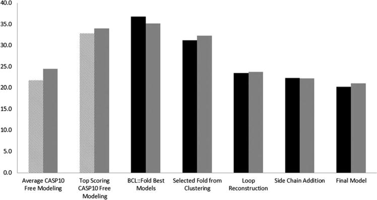
GDT_TS score analysis. Twenty FM targets from CASP10 (left two bars, pattern). Three targets folded also by BCL::Fold from FM category in CASP10 (left two bars, gray). All 18 targets folded by BCL::Fold (black). Three FM targets folded by BCL::Fold (right five bars, gray). The y axis represents GDT_TS score.

Quality of BCL::Fold models and sampling of the topology space

We assess the quality of BCL::Fold models in two ways. The GDT_TS score allows for comparison with other results; the topology score focuses its evaluation criteria specifically on SSE contacts which tests BCL::Fold’s method of assembly.

GDT_TS scores for the best model generated by BCL::Fold ranged in from 23.3 to 64.5% with a mean GDT_TS score of 36.8% and a standard deviation of 10.4%. Using the mean GDT_TS score of 33% as a comparative measure between other methods, BCL::Fold was able to sample models above this threshold in 12 out of 18 cases. Comparisons of the BCL models with the experimentally determined structure by measuring RMSD100⁴⁹ and GDT_TS show efficient sampling of the correct topology (Table IV, Fig. 3).

Table IV.

Comparison of the GDT_TS Score and RMSD100 Score with the Native Showing the Best Model Produced During Folding with BCL::Fold (A); The Selected Models from Clustering (B); The Models After Loop Reconstruction (C); The Models After Side Chain Addition (D); The Final Submitted Model (E)

Target	PDB ID	GDT_TS					RMSD 100
		A	B	C	D	E	A	B	C	D	E
T0644	4FR9	41.7	32.1	19.1	21.1	21.1	7.7	12.4	11.5	10.5	10.5
T0649	4F54	38.5	29.5	19.5	16.7	12.6	9.6	13.5	14.8	14.9	14.9
T0655	2LUZ	37.4	25.6	18.1	18.0	17.0	9.6	13.4	10.4	11.2	11.2
T0663	4EXR	43.0	39.7	26.0	24.7	24.5	5.8	7.1	10.2	13.1	13.3
T0666	3UX4	38.8	35.0	29.9	28.6	25.6	5.1	7.2	6.9	7.1	8.3
T0676	4E6F	31.9	26.2	24.0	21.3	20.0	9.7	11.7	11.6	13.1	13.1
T0678	4EPZ	40.0	29.1	30.7	29.2	20.9	8.0	10.3	7.9	11.5	11.8
T0682	4JQ6	37.4	28.8	37.1	36.3	33.0	4.8	8.3	4.5	4.6	5.4
T0684	4GL6	23.8	22.2	15.3	13.5	13.1	12.0	12.0	12.8	13.7	13.7
T0686	4JQ6	29.1	29.1	13.8	12.0	12.0	10.4	10.4	12.2	16.9	16.9
T0691	4GZV	34.8	26.8	19.2	17.4	13.7	10.9	12.7	10.9	12.3	15.2
T0700	4HFX	64.5	57.6	38.6	38.6	31.3	7.2	10.4	14.1	13.3	15.4
T0704	4HG2	25.0	17.9	12.6	11.3	10.5	10.7	11.9	10.3	13.5	13.5
T0720	4IC1	26.1	24.2	19.8	19.8	15.6	10.6	10.8	10.3	10.8	13.8
T0722	4FLA	53.5	46.0	38.7	40.7	38.9	5.1	6.9	20.7	20.1	21.7
T0724	4FMR	23.3	21.9	13.6	12.4	12.4	11.8	14.1	14.4	17.3	17.3
T0743	4HYZ	38.4	37.2	25.7	25.2	23.5	8.3	10.6	9.4	9.8	10.6
T0745	4FMW	35.1	33.1	21.8	18.7	18.5	8.5	10.2	10.4	11.5	14.0

FM Target	Average GDT_TS	Best GDT_TS
T0663	36	43.5
T0666	21	34
T0684	16.5	24.5

Figure 3.

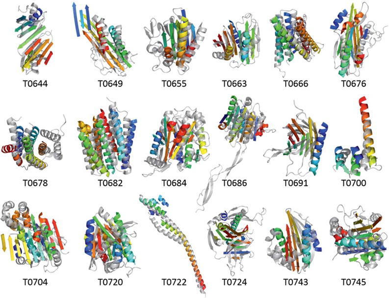
Highest GDT_TS model sampled with BCL::Fold (rainbow) overlaid with experimental protein structure (gray).

BCL::Fold’s sampling performance was evaluated previously with soluble and membrane proteins. BCL::Fold was able to sample the correct topology in 61 of 66 soluble benchmark proteins²² and in 32 of 38 membrane benchmark proteins.⁶ The correct topology was defined as the ability to fold models with an RMSD100 of <8 Å to the native.

While RMSD100 is suitable to assess Rosetta models, it is not as helpful for BCL::Fold models that are focusing on sampling long-range contacts between SSEs. Figure 4 shows how well BCL::Fold samples the different protein topologies, measured the topology score. Its applicability is limited foremost by the number of SSE contacts. For targets with very few contacts (T0722 has a single contact) many models achieve a high score, and the discriminative value of the topology score is reduced. While the topology score does currently not consider specific types of interactions between SSEs, it does include the secondary structure type; thus, an incorrectly predicted secondary structure type leads to all contacts of this incorrect SSE to be evaluated as false. The thresholds to assume a contact between two SSEs are derived from idealized, native protein models and therefore fairly large; this can lead to detection of SSE contacts even for SSEs that are only indirectly in contact but still a very short Euclidean distance apart, like the first and third strand of a sheet. Additionally, the value of the topology visualization is narrowed by the projection of three-dimensional protein structures into two dimensions, which reaches its limits for complex topologies. While the topology score has some caveats, overall it captures the protein topology quite well.

For the topology score, which measures the true positive contact ratio, we set the threshold to 0.8. At this level, two topologies share an overwhelming number of SSE contacts. Furthermore, we observe similarities when visually inspecting the topology plots of protein models (Fig. 4).

BCL::Fold samples models above the threshold of 0.8 for 11 out of 18 targets (Fig. 5). All targets with a native SSE contact count up to 20 have a topology score above the threshold. With increasing native SSE contact count and complexity, the topology score decreases expectedly.

Figure 5.

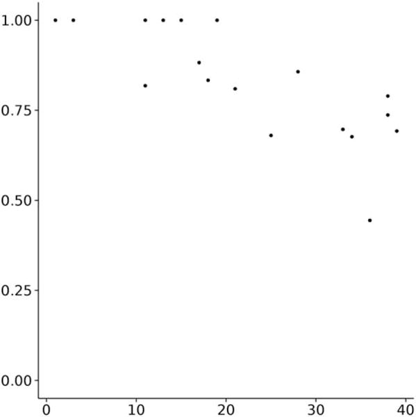
True positive rate (precision, y axis) compared with the complexity of a protein (number of SSE contacts in the native, x axis). The true positive rate of BCL::Fold models decreases with increasing complexity.

Selection of models for loop and side chain construction

Difficult, however, proved the selection of models for the subsequent refinement steps. During CASP10 we attempted selecting the best models by BCL sum score, the centers of the largest clusters, and the best scoring models in each cluster. However, no method enriched for high GDT_TS and consequently the models most similar to the native were consistently lost. For model T0700, we sampled a topology with an overall GDT_TS score of 64.5. We selected a model with a GDT_TS score of 57.6 for further refinement. After loop and side chain reconstruction, our model drifted further from the true native structure with a GDT_TS score of 38.6. Our final submitted model for this target had a GDT_TS score of 31.3. Most of the targets folded with BCL::Fold had this attrition pattern. Interestingly, model T0682 improved substantially after loop reconstruction from a GDT_TS score of 28.8 to 37.1. Our final submitted to CASP10 for this target had an RMSD100 score of 5.4 and GDT_TS Score of 33.0 (Figs. 2 and 6).

Figure 6.

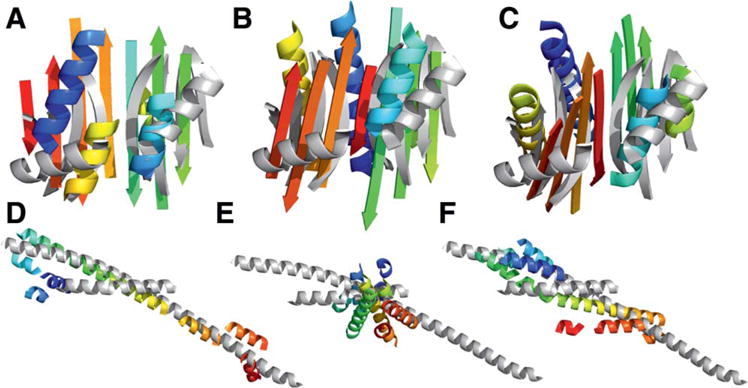
Comparison of example BCL models with the native target structure for T0663 (top) and T0722 (bottom). The experimental structures without loops are shown in gray (based on PDBIDs 4EXR and 4FLA, respectively). The predicted models (rainbow) show the highest scoring model produced by BCL (A, D, with a GDT_TS of 43.0 and 53.5, respectively); The best scoring model by BCL energy function (B, E, with a GDT_TS of 28.9 and 26.9); The best scoring model in largest cluster (C, F, with a GDT_TS of 22.1 and 32.6). [Color figure can be viewed in the online issue, which is available at wileyonlinelibrary.com.]

Addition of loop and side chain coordinates

While adding loops to the cluster centers decreased the average GDT_TS scores from 31.2 to 23.5, the GDT_TS average dropped again from 23.5 to 22.4 when the side chains were added with Rosetta version 3.3. To rebuild side chains, the models were relaxed. To limit movement of the backbone constraints for every C_α-C_α bond distance below a cutoff of 8 Å were applied using a harmonic function with a standard deviation of 0.5. During side-chain reconstruction with Rosetta, 12 of the 18 CASP10 targets had a radius of gyration score >1100 for approximately 30% of all models indicating unfolding despite the constraint used (T0644, T0649, T0655, T0663, T0666, T0684, T0691, T0704, T0720, T0722, T0743, and T0745). This unfolding-like event was triggered because the BCL models scored poorly in the Rosetta energy function (Fig. 7). Models that were unfolded were not considered further. As a method of last resort, Rosetta was used to add side chains without relaxing the backbone but only repacking the side chains.

Figure 7.

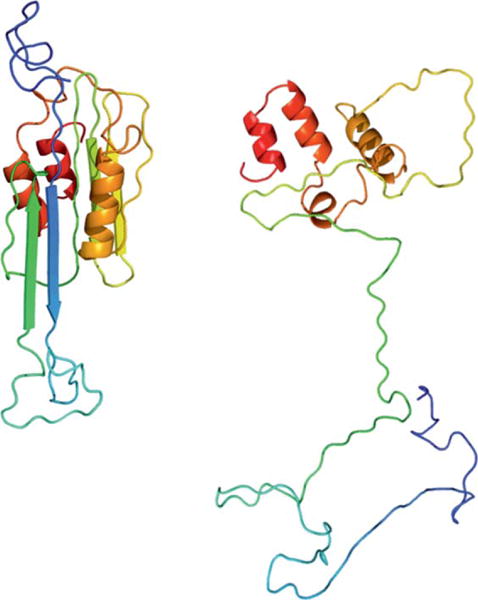
BCL model for target T0655 before (A) and after side chain addition and relaxation with Rosetta (B). [Color figure can be viewed in the online issue, which is available at wileyonlinelibrary.com.]

DISCUSSION

BCL::Fold fails to sample to correct topology in seven cases

In 7 out of 18 cases, the best scoring BCL::Fold model had a topology score of <0.8, which means the correct topology was not found. Investigating the reasons for these failures, we found that the target with the lowest topology scores had SSEs missing in the secondary structure prediction and subsequently in the SSE pool. T0655 had a topology score of 0.44 and had two helices missing; T0649 had a score of 0.68 and had one helix missing.

Models for T0724 have an incorrect strand topology because BCL::Fold models were created as protomers while the native exists as dimer in which strands from both monomers form a sheet.

The remainder of four incorrect targets failed to sample the correct topology because of a combination of reasons, most notably for two reasons. Long SSEs were split into two smaller ones, either by DSSP when assigning secondary structure to the natives, or by the secondary structure prediction methods that we employed. The correct topology was simply not sampled and recognized as a best scoring model, often with the order of strand SSEs in sheets being incorrect.

BCL::Fold models have loops that are impossible to close

BCL::Fold assembles tertiary structure from disconnected SSEs. Because of this, we must ensure that the distance between the end of one SSE and the beginning of the next SSE can be bridged by a loop. Two components of the BCL::Fold scoring function control this requirement: First, there is a penalty if the Euclidean distance between two SSEs is longer than the maximal Euclidean distance that can be bridged by the number of amino acids in the loop. Models that violate this rule are heavily penalized during Monte Carlo sampling and likely rejected. The second component is designed to place SSEs so that loops between them match a loop score potential that reflects native loop conformations from the PDB (PISCES dataset, see Methods). This loop score potential evaluates the Euclidean distance probability in dependence of number of residues.²³ As this score is a function of only Euclidean distance and sequence distance, it neglects the spatial arrangement of SSEs. Analysis of CASP10 models revealed that BCL::Fold constructs models where loops cannot be closed without passing through SSEs. Figure 8 depicts a model produced by BCL::Fold for target T0663. The Euclidean distance between residues ASN55 of helix 1 and TYR65 of helix 2 is 25.5 Å. To bridge this distance with 9 amino acids, each amino acid has to be 2.8 Å on average, which is less than the average C_α-C_α distance of 3.3 Å. However, with the placement of strand SSEs between the loop ends, all paths to close the loop between helices 1 and 2 pass through the strand SSEs. Overall, 76% of BCL::Fold models produced during CASP10 folding simulations contains nonclosable loops because of this behavior.

Figure 8.

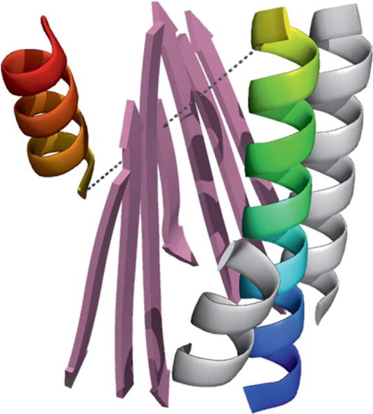
A model for CASP10 target T0663 folded by BCL. The Euclidean distance between residues ASN55 in helix 1 (rainbow colored on the right) and TYR65 in helix 2 (rainbow colored on the left) is 25.5 Å. Without the central sheet (pink) the loop could be closed; it is impossible to close the loop if the connecting amino acids have to be positioned around the sheet. [Color figure can be viewed in the online issue, which is available at wileyonlinelibrary.com.]

The BCL::Fold loop potential is often violated for consecutive SSEs

Loops found in native proteins bridge preferable Euclidean distances d_e depending on the loop’s sequence length d_s. The current loop potential of BCL::Fold mirrors this preference. It is a sequence independent score, which contributes to the overall energy function. The PISCES data set used to create this potential includes all possible loops, that is, loops between consecutive and nonconsecutive SSEs. Because BCL::Fold does not assemble SSEs in sequence order, the potential must evaluate incomplete protein models with unplaced SSEs. Therefore, nonconsecutive SSEs were included in the loop scoring potential.

To test the loop potential accuracy, we compare the CASP10 models produced by BCL::Fold to structures from the PISCES pdb set. Because the Euclidean distance that a loop spans depends on the sequence length of the loop, we normalize the Euclidean distance by the logarithm of the sequence length, d_e/logd_s; this results in homogeneous distributions independent of loop length. The all-loop distributions (that is, consecutive and non-consecutive loops) for d_e/logd_s for CASP10 models, CASP10 natives, and PISCES are alike [Fig. 9(A)]. The means of the distributions are 6.2, 6.6, and 6.5 Å, respectively, and confirm their similarity. Thus, we conclude that this weighted potential distinguishes native-like sequence and distance length of loops from non-native configurations in terms of sequence length and corresponding Euclidean distance.

Figure 9.

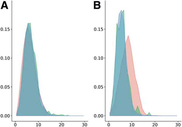
The density distribution of the BCL loop score displaying Euclidean distance over the logarithm of the sequence separation for loop regions between all SSEs (A) and consecutive SSEs only (B). While the distributions of BCL models (red), CASP10 natives (green) and PISCES dataset (blue) match each other for loops between all SSEs (A), the distribution of BCL models shows a shift when only loops between consecutive SSEs are considered (B). [Color figure can be viewed in the online issue, which is available at wileyonlinelibrary.com.]

However, when evaluating the CASP10 models with the consecutive-only loop distribution (that is, only loops between consecutive SSEs are included), we find a substantial bias between CASP10 models and both CASP10 natives and PISCES structures [Fig. 9(B)]. Their means are 8.1, 5.8, and 5.7 Å, respectively. The sequence length d_s of a loop is not changing as it is defined by the secondary structure (prediction) of the particular protein and only used for normalization. Therefore, the difference between the distributions can only be caused by differences in the Euclidean distances d_e. Creating models with loops of longer Euclidean distances d_e than found in native structures for a given sequence length causes BCL::Fold to produce non-native like loop arrangements. Thus, the loop potential is not a sufficient metric to generate native-like models from disconnected SSEs. Furthermore, the current loop potential does not consider the spatial positioning of other SSEs and does not account for potential clashes between these SSEs and a loop (Fig. 8).

A small loop angle favors more native-like loops

To address the shortcoming we devised a loop measure that reflects this difference between consecutive and non-consecutive SSEs more drastically. For native proteins, we observe that loops between consecutive SSEs are positioned locally on a protein structure, that is, consecutive loops tend to begin and end on the same side of the structure and do not connect through the center. Geometrically this can be measured at as the angle between the end of one helix, the center of the protein, and the start of the next helix [Fig. 10(A)]. In native protein structures, consecutive loops overwhelmingly favor small angles, as shown for the CASP10 native and PISCES pdb sets, of which 75% are smaller than 40° [Fig. 10(B) green and blue, respectively]. Models with loops that would clash with other parts of the protein frequently have large angles of close to 180° [Fig. 10(B), red]. We can use this information to discriminate native like arrangements from models with large angles.

Figure 10.

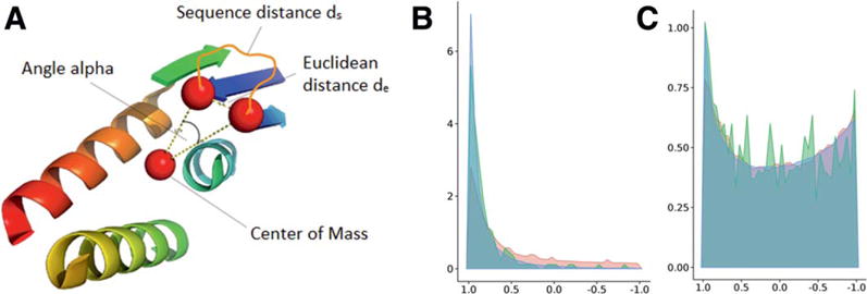
Visualization of loop angle metric, which measures the angle α between the end of one SSE (dark blue), the center of gravity, and the beginning of the next SSE (light blue; A). The density distribution of the cos(α) metric for loop regions between consecutive SSEs only is concentrated to acute angles for PISCES and CASP10 natives (B, blue and red, respectively). BCL models exhibit a higher number of large angles for consecutive loops (B, red). The density distribution of the cos(α) metric for loop regions between all possible SSEs shows two frequently found angles, small ones and large ones, for all sets, BCL models (red), CASP10 natives (green) and PISCES (blue; C). [Color figure can be viewed in the online issue, which is available at wileyonlinelibrary.com.]

When including nonconsecutive loops, the distribution of loop angles is exhibiting two frequently occurring angles, small ones for loops connecting consecutive SSEs, and large ones for connecting nonconsecutive SSEs [Fig. 10(C)]. To evaluate the loop angles of a protein model, we must differentiate between loops that connect consecutive and nonconsecutive SSEs.

To test whether filtering by the new loop angle measure would select for lower RMSD models compared to the existing loop score, we folded models for eight CASP10 targets (1000 models for T0655, T0663, T0676, T0678, T0684, T0700, T0745; 700 models for T0722). The RMSD cutoff was set to 10th percentile. Both, the existing loop score and the loop angle score were then used to select the best 50% according to each score. The existing loop score filtered on average 50% of the models below the RMSD cutoff and in three cases decreased the number of models below the RMSD cutoff by more than the expected 50% (T0684, T0700, and T0722). The loop angle score filtered on average 61% of the models below the RMSD cutoff and only in one case, T0722, it selected less than 50% of the models below the RMSD cutoff. Thus, the loop angle score is selecting more native-like models and can improve the BCL scoring function moving forward (Table V).

Table V.

The Percentage of Models Below the RMSD Cutoff Kept When Filtering Models for Each Target with the Existing Loop Score and the Loop Angle Score, Showing that the Loop Angle Score Keeps in All Cases More Low RMSD Models

Target	% Models kept by existing loop score	% Models kept by loop angle score
T0655	70	70
T0663	67	76
T0676	52	57
T0678	52	63
T0684	44	57
T0700	37	57
T0722	16	43
T0745	59	62
Average	50	61

BCL::Fold misaligns β-strand registers

Carbonyl and amide groups in parallel and antiparallel strands of native proteins are aligned to allow the formation of stabilizing hydrogen bonds. A hydrogen bond is formed between the carbonyl-oxygen (hydrogen-bond acceptor) of one amino acid with the amide hydrogen of another amino acid (donor). In a sheet with the antiparallel strands i and j, the following pairs of atoms form hydrogen-bonds, here denoted as (acceptor, donor): (C_i, C_j), (C_j, C_i), (C_i+2, C_j−2), (C_j−2, C_i+2), (C_i+4, C_j−4), (C_j−4, C_i+4),… [Fig. 11(A)]; the pattern for parallel strands i and j is:(C_i, C_j+1), (C_j+1, C_i+2), (C_i+2, C_j+3),… [Fig. 11(C)].

Figure 11.

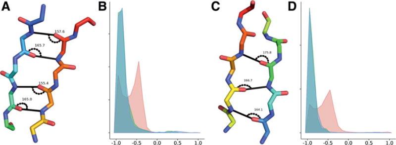
Hydrogen-bond pattern and angles between the carbonyl-carbon, carbonyl-oxygen, and amide-hydrogen in antiparallel (A) and parallel strands (C). Comparison of the hydrogen-bond angle for BCL models (red), CASP10 natives (green), and PISCES (blue) for antiparallel (B) and parallel strands (D). While the angles for CASP10 native and PISCES sets match, BCL models deviate. The x axis shows the cosine of the hydrogen-bond angle, the y axis the normalized density. [Color figure can be viewed in the online issue, which is available at wileyonlinelibrary.com.]

BCL::Fold does not control for this alignment in order to simplify the folding energy landscape. It only controls for distance and relative orientation of β-strands within β-sheets. We hypothesized that misalignment of hydrogen bonds within β-sheets might cause clashes that are responsible for the large fraction of models that unfolds during Rosetta refinement.

To evaluate the strand register alignment of BCL models and compare them to natives, we measured the angle between carbonyl-carbon, the carbonyl-oxygen and the amide-hydrogen, and the distance from the carbonyl-oxygen to the amide-hydrogen. While in native proteins a hydrogen bond rarely has a Euclidean distance longer than 2.1 Å, we measured putative hydrogen bond atom pairs that were in paired β-strand SSEs and within a relaxed cutoff of 4.5 Å. The hydrogen-bonds in aligned strands of elucidated proteins have characteristic angles close to 180° and distances of 1.9 to 2 Å. Analysis of CASP10 BCL::Fold models, CASP10 experimental structures, and the PISCES is summarized in Figure 11. In BCL models, we find substantial deviations to smaller angles and larger distances up to 4 Å for more than half of the models for both antiparallel and parallel sheets. The deviation in hydrogen bond angle and distance is correlated in BCL models. Additionally, BCL models exhibit a slightly shorter hydrogen bond distance of 1.8 to 1.9 Å even for hydrogen bonds with a native-like angle (Supporting Information Fig. S1). This points to an incorrect placement of SSEs.

Misaligned β-strands cause clashes in Rosetta

The misaligned β-strands result in a high positive contribution from the repulsive score term (fa_rep) and no attractive contribution from the hydrogen bond score term (hbond_lr_bb), which leads to an unfavorable Rosetta score overall. The fa_rep term is the repulsive component of the van der Waals force, for example originating from carbonyl-oxygen of two strands being positioned too close to each other. The hbond_lr_bb term evaluates backbone-backbone hydrogen bonds distant in the primary sequence as they appear in sheets. Due to the misalignment of strands, the hbond_lr_bb term is zero and does not contribute to the overall Rosetta score (Fig. 12).

Figure 12.

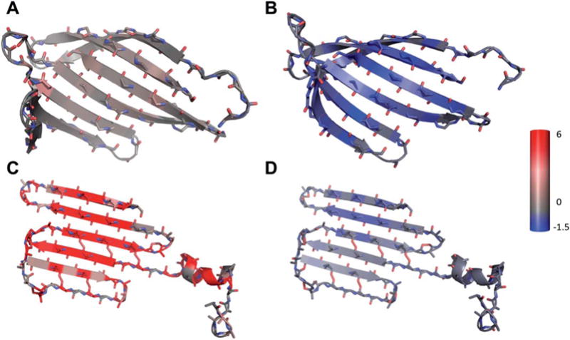
The analysis of Rosetta energy scoring terms for the native and a BCL model of target T0655 (shown is only the sheet part of native and model). The native shows no penalty from the repulsive score (A, fa_rep Rosetta score term) and a beneficial contribution from the hydrogen bonding score term (B, hbond_lr_bb Rosetta score term). Contrary, the BCL model exhibits a very high repulsive score (C, fa_rep) and little benefit from the hydrogen bonding term (D, hbond_lr_bb). The color scale stretches from blue representing −1.5 Rosetta energy units (REU) through gray (0 REU) to red (6 REU); the scale was chosen to red depict a value further from zero than blue to account for the bigger range of the repulsive score.

This causes Rosetta to unfold BCL models, despite constraints (Fig. 7), in the last step of our CASP10 pipeline, which adds side chains and structurally refines the protein by cycling through repack and minimization steps.

β-Strand placement in BCL::Fold models needs to be refined to align hydrogen bond donors and acceptors

The assembly of disconnected SSEs allows BCL::Fold to sample different sheet topologies and register positions without being restricted by the residues connecting the two strand SSEs. For this reason β-strand placement is controlled only by a mutate-function that places one strand next to another in the preferred angle and distance.²³ However, the placement of β-strands only by the distance and torsion angle within the β-sheet is insufficient to produce BCL::Fold models that can be refined with other programs. We plan to add a refinement stage into BCL::Fold that translates β-strands along their z-axis and evaluates a scoring term that controls the angle α introduced above. This will result in an improved scoring function that selects for more native-like models. We expect that improved alignment of β-strands will reduce the unfolding events observed during Rosetta refinement.

CONCLUSION

Despite inaccuracies in secondary structure prediction, BCL::Fold was able to sample the correct fold for most of 18 cases studied herein. The best methods in CASP10 submitted models with an average GDT_TS of around 33% in the FM category. BCL::Fold achieves this threshold in initial models after folding for 12 of 18 targets. Similarly, BCL::Fold is able to produce models with a topology score of at least 0.8 for 11 of 18 targets. However, the post folding filtering and refinement strategies removed correctly folded models from consideration in almost all cases, mostly for structural artefacts present in the BCL::Fold models. This result shows that BCL::Fold has the potential to compete with the best de novo structure prediction algorithms if a) unrealistic geometries in loops and β-strands can be removed and thereby the attrition of accurate topologies during model refinement can be stopped and b) an approach can be found that recognizes the most accurate models within the BCL::Fold ensemble. However, with this analysis and planned work to address the recognized weaknesses, future versions of BCL::Fold produce more native-like models without incorporating templates or experimental data.

References

- 1.Berman HM. The protein data bank. Nucleic Acids Res. 2000;28:235–242. doi: 10.1093/nar/28.1.235. [DOI] [PMC free article] [PubMed] [Google Scholar]
- 2.Berman HM. The protein data bank: a historical perspective. Acta Crystallogr A. 2008;64:88–95. doi: 10.1107/S0108767307035623. [DOI] [PubMed] [Google Scholar]
- 3.Dutta S, Berman HM. Large macromolecular complexes in the protein data bank: a status report. Structure. 2005;13:381–388. doi: 10.1016/j.str.2005.01.008. [DOI] [PubMed] [Google Scholar]
- 4.Bill RM, Henderson PJ, Iwata S, Kunji ER, Michel H, Neutze R, Newstead S, Poolman B, Tate CG, Vogel H. Overcoming barriers to membrane protein structure determination. Nat Biotechnol. 2011;29:335–340. doi: 10.1038/nbt.1833. [DOI] [PubMed] [Google Scholar]
- 5.Hopf TA, Colwell LJ, Sheridan R, Rost B, Sander C, Marks DS. Three-dimensional structures of membrane proteins from genomic sequencing. Cell. 2012;149:1607–1621. doi: 10.1016/j.cell.2012.04.012. [DOI] [PMC free article] [PubMed] [Google Scholar]
- 6.Weiner BE, Woetzel N, Karakas M, Alexander N, Meiler J. BCL::MP-fold: folding membrane proteins through assembly of transmembrane helices. Structure. 2013;21:1107–1117. doi: 10.1016/j.str.2013.04.022. [DOI] [PMC free article] [PubMed] [Google Scholar]
- 7.Alber F, Dokudovskaya S, Veenhoff LM, Zhang W, Kipper J, Devos D, Suprapto A, Karni-Schmidt O, Williams R, Chait BT, Rout MP, Sali A. Determining the architectures of macromolecular assemblies. Nature. 2007;450:683–694. doi: 10.1038/nature06404. [DOI] [PubMed] [Google Scholar]
- 8.Anfinsen CB. Principles that govern the folding of protein chains. Science. 1973;181:223–230. doi: 10.1126/science.181.4096.223. [DOI] [PubMed] [Google Scholar]
- 9.Crippen GM. Global optimization and polypeptide conformation. J Comput Phys. 1975;18:224–231. [Google Scholar]
- 10.Chivian D, Kim DE, Malmstrom L, Schonbrun J, Rohl CA, Baker D. Prediction of CASP6 structures using automated robetta protocols. Proteins. 2005;61:157–166. doi: 10.1002/prot.20733. [DOI] [PubMed] [Google Scholar]
- 11.Leaver-Fay A, Tyka M, Lewis SM, Lange OF, Thompson J, Jacak R, Kaufman K, Renfrew PD, Smith CA, Sheffler W, et al. ROSETTA3: An object-oriented software suite for the simulation and design of macromolecules. Methods Enzymol. 2011;487:545–574. doi: 10.1016/B978-0-12-381270-4.00019-6. [DOI] [PMC free article] [PubMed] [Google Scholar]
- 12.Simons KT, Kooperberg C, Huang E, Baker D. Assembly of protein tertiary structures from fragments with similar local sequences using simulated annealing and bayesian scoring functions. J Mol Biol. 1997;268:209–225. doi: 10.1006/jmbi.1997.0959. [DOI] [PubMed] [Google Scholar]
- 13.Bradley P, Misura KM, Baker D. Toward high-resolution de novo structure prediction for small proteins. Science. 2005;309:1868–1871. doi: 10.1126/science.1113801. [DOI] [PubMed] [Google Scholar]
- 14.Bradley P, Malmstrom L, Qian B, Schonbrun J, Chivian D, Kim DE, Meiler J, Misura KM, Baker D. Free modeling with rosetta in CASP6. Proteins. 2005;61:128–134. doi: 10.1002/prot.20729. [DOI] [PubMed] [Google Scholar]
- 15.Kaufmann KW, Lemmon GH, Deluca SL, Sheehan JH, Meiler J. Practically useful: what the rosetta protein modeling suite can do for you. Biochemistry. 2010;49:2987–2998. doi: 10.1021/bi902153g. [DOI] [PMC free article] [PubMed] [Google Scholar]
- 16.Baker D. A surprising simplicity to protein folding. Nature. 2000;405:39–42. doi: 10.1038/35011000. [DOI] [PubMed] [Google Scholar]
- 17.Grantcharova V, Alm EJ, Baker D, Horwich AL. Mechanisms of protein folding. Curr Opin Struct Biol. 2001;11:70–82. doi: 10.1016/s0959-440x(00)00176-7. [DOI] [PubMed] [Google Scholar]
- 18.Bonneau R, Ruczinski I, Tsai J, Baker D. Contact order and ab initio protein structure prediction. Protein Sci. 2002;11:1937–1944. doi: 10.1110/ps.3790102. [DOI] [PMC free article] [PubMed] [Google Scholar]
- 19.Wu S, Skolnick J, Zhang Y. Ab initio modeling of small proteins by iterative TASSER simulations. BMC Biol. 2007;5:17. doi: 10.1186/1741-7007-5-17. [DOI] [PMC free article] [PubMed] [Google Scholar]
- 20.Zhang Y. Interplay of I-TASSER and QUARK for template-based and ab initio protein structure prediction in CASP10. Proteins. 2014;82:175–187. doi: 10.1002/prot.24341. [DOI] [PMC free article] [PubMed] [Google Scholar]
- 21.Zhang Y. Template-based modeling and free modeling by I-TASSER in CASP7. Proteins. 2007;69:108–117. doi: 10.1002/prot.21702. [DOI] [PubMed] [Google Scholar]
- 22.Karakas M, Woetzel N, Staritzbichler R, Alexander N, Weiner BE, Meiler J. BCL::fold–de novo prediction of complex and large protein topologies by assembly of secondary structure elements. PLoS One. 2012;7:e49240. doi: 10.1371/journal.pone.0049240. [DOI] [PMC free article] [PubMed] [Google Scholar]
- 23.Woetzel N, Karakas M, Staritzbichler R, Muller R, Weiner BE, Meiler J. BCL::score–knowledge based energy potentials for ranking protein models represented by idealized secondary structure elements. PLoS One. 2012;7:e49242. doi: 10.1371/journal.pone.0049242. [DOI] [PMC free article] [PubMed] [Google Scholar]
- 24.Baker D, Sali A. Protein structure prediction and structural genomics. Science. 2001;294:93–96. doi: 10.1126/science.1065659. [DOI] [PubMed] [Google Scholar]
- 25.Rohl CA, Strauss CE, Chivian D, Baker D. Modeling structurally variable regions in homologous proteins with rosetta. Proteins. 2004;55:656–677. doi: 10.1002/prot.10629. [DOI] [PubMed] [Google Scholar]
- 26.Sali A, Blundell TL. Comparative protein modelling by satisfaction of spatial restraints. J Mol Biol. 1993;234:779–815. doi: 10.1006/jmbi.1993.1626. [DOI] [PubMed] [Google Scholar]
- 27.Rost B. PHD: predicting one-dimensional protein structure by profile-based neural networks. Methods Enzymol. 1996;266:525–539. doi: 10.1016/s0076-6879(96)66033-9. [DOI] [PubMed] [Google Scholar]
- 28.Rost B, Sander C. Combining evolutionary information and neural networks to predict protein secondary structure. Proteins. 1994;19:55–72. doi: 10.1002/prot.340190108. [DOI] [PubMed] [Google Scholar]
- 29.Jones DT. Protein secondary structure prediction based on position-specific scoring matrices. J Mol Biol. 1999;292:195–202. doi: 10.1006/jmbi.1999.3091. [DOI] [PubMed] [Google Scholar]
- 30.Ward JJ, McGuffin LJ, Buxton BF, Jones DT. Secondary structure prediction with support vector machines. Bioinformatics. 2003;19:1650–1655. doi: 10.1093/bioinformatics/btg223. [DOI] [PubMed] [Google Scholar]
- 31.Leman JK, Mueller R, Karakas M, Woetzel N, Meiler J. Simultaneous prediction of protein secondary structure and transmembrane spans. Proteins. 2013;81:1127–1140. doi: 10.1002/prot.24258. [DOI] [PMC free article] [PubMed] [Google Scholar]
- 32.Meiler J, Baker D. Coupled prediction of protein secondary and tertiary structure. Proc Natl Acad Sci USA. 2003;100:12105–12110. doi: 10.1073/pnas.1831973100. [DOI] [PMC free article] [PubMed] [Google Scholar]
- 33.Meiler J, Muller M, Zeidler A, Schmaschke F. Generation and evaluation of dimension-reduced amino acid parameter representations by artificial neural networks. J Mol Model. 2001;7:360–369. [Google Scholar]
- 34.Viklund H, Bernsel A, Skwark M, Elofsson A. SPOCTOPUS: a combined predictor of signal peptides and membrane protein topology. Bioinformatics. 2008;24:2928–2929. doi: 10.1093/bioinformatics/btn550. [DOI] [PubMed] [Google Scholar]
- 35.Viklund H, Elofsson A. OCTOPUS: improving topology prediction by two-track ANN-based preference scores and an extended topological grammar. Bioinformatics. 2008;24:1662–1668. doi: 10.1093/bioinformatics/btn221. [DOI] [PubMed] [Google Scholar]
- 36.Wang G, Dunbrack RL., Jr PISCES: recent improvements to a PDB sequence culling server. Nucleic Acids Res. 2005;33:W94–98. doi: 10.1093/nar/gki402. (Web Server issue) [DOI] [PMC free article] [PubMed] [Google Scholar]
- 37.Wang G, Dunbrack RL., Jr PISCES: a protein sequence culling server. Bioinformatics. 2003;19:1589–1591. doi: 10.1093/bioinformatics/btg224. [DOI] [PubMed] [Google Scholar]
- 38.Moult J. A decade of CASP: progress, bottlenecks and prognosis in protein structure prediction. Curr Opin Struct Biol. 2005;15:285–289. doi: 10.1016/j.sbi.2005.05.011. [DOI] [PubMed] [Google Scholar]
- 39.Moult J, Fidelis K, Kryshtafovych A, Tramontano A. Critical assessment of methods of protein structure prediction (CASP)–round IX. Proteins. 2011;79:1–5. doi: 10.1002/prot.23200. [DOI] [PMC free article] [PubMed] [Google Scholar]
- 40.Taylor TJ, Bai H, Tai CH, Lee B. Assessment of CASP10 contact-assisted predictions. Proteins. 2014;82:84–97. doi: 10.1002/prot.24367. [DOI] [PMC free article] [PubMed] [Google Scholar]
- 41.Monastyrskyy B, D’Andrea D, Fidelis K, Tramontano A, Kryshtafovych A. Evaluation of residue-residue contact prediction in CASP10. Proteins. 2014;82:138–153. doi: 10.1002/prot.24340. [DOI] [PMC free article] [PubMed] [Google Scholar]
- 42.Nugent T, Cozzetto D, Jones DT. Evaluation of predictions in the CASP10 model refinement category. Proteins. 2014;82:98–111. doi: 10.1002/prot.24377. [DOI] [PMC free article] [PubMed] [Google Scholar]
- 43.Kryshtafovych A, Barbato A, Fidelis K, Monastyrskyy B, Schwede T, Tramontano A. Assessment of the assessment: evaluation of the model quality estimates in CASP10. Proteins. 2014;82:112–126. doi: 10.1002/prot.24347. [DOI] [PMC free article] [PubMed] [Google Scholar]
- 44.Zemla A, Venclovas C, Moult J, Fidelis K. Processing and analysis of CASP3 protein structure predictions. Proteins. 1999:22–29. doi: 10.1002/(sici)1097-0134(1999)37:3+<22::aid-prot5>3.3.co;2-n. [DOI] [PubMed] [Google Scholar]
- 45.Ginalski K, Elofsson A, Fischer D, Rychlewski L. 3D-jury: a simple approach to improve protein structure predictions. Bioinformatics. 2003;19:1015–1018. doi: 10.1093/bioinformatics/btg124. [DOI] [PubMed] [Google Scholar]
- 46.Canutescu AA, Dunbrack RL., Jr Cyclic coordinate descent: a robotics algorithm for protein loop closure. Protein Sci. 2003;12:963–972. doi: 10.1110/ps.0242703. [DOI] [PMC free article] [PubMed] [Google Scholar]
- 47.Fischer A, Alexander N, Woetzel N, Karakas M, Weiner B, Meiler J. BCL::MP-fold: membrane protein structure prediction guided by EPR restraints. Structure, Submitted. doi: 10.1002/prot.24801. [DOI] [PMC free article] [PubMed] [Google Scholar]
- 48.Ortiz AR, Strauss CE, Olmea O. MAMMOTH (matching molecular models obtained from theory): an automated method for model comparison. Protein Sci. 2002;11:2606–2621. doi: 10.1110/ps.0215902. [DOI] [PMC free article] [PubMed] [Google Scholar]
- 49.Carugo O, Pongor S. A normalized root-mean-square distance for comparing protein three-dimensional structures. Protein Sci. 2001;10:1470–1473. doi: 10.1110/ps.690101. [DOI] [PMC free article] [PubMed] [Google Scholar]
Associated Data
This section collects any data citations, data availability statements, or supplementary materials included in this article.