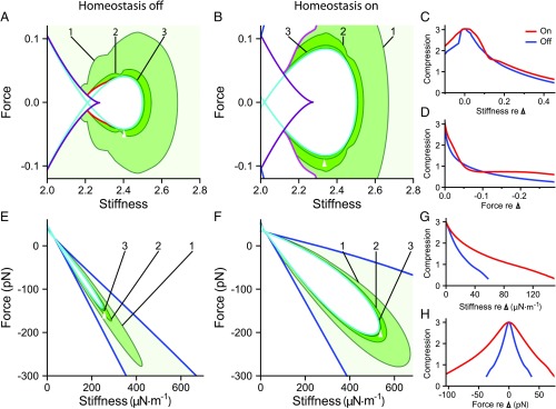
Fig. 5.

Homeostasis increases the robustness of a hair bundle’s dynamic range. ($A$) A contour plot showing curves of constant compressive range for model I when homeostasis is off. ($A$ and $B$) Compressive range is shown as a function of the stiffness (abscissa) and constant force (ordinate). The contour labels indicate the size of the compressive range in orders of magnitude of the periodic forcing amplitude; see Fig. 4 for examples. Darker shades of green indicate broader compressive ranges. The purple curve is a line of saddle-node bifurcations; saddle-node bifurcations of limit cycles are colored red. ($B$) A contour plot of compressive range when homeostasis is on. Multimodal oscillations occur in response to sinusoidal forcing within the region on the left-hand side of the magenta curves. The purple curve is a line of saddle-node bifurcations. The apices of the white triangles indicate the reference operating points through which horizontal and vertical slices are taken to generate the curves for $C$ and $D$, respectively. ($E$–$H$) Compressive range for model II when homeostasis is inactive $(E)$ or active $(F)$. $G$ and $H$ show the compressive range of the bundle along either a horizontal $(G)$ or vertical $(H)$ slice through the apices of the white triangles in $E$ and $F$. The Hopf bifurcation curve is colored cyan in each contour plot, and the blue curve marks the boundary of the underdamped region of the state diagrams. At each operating point, sinusoidal stimuli are delivered at the bundle’s resonant frequency, which varies as a function of stiffness and constant force. The stimulus frequency is not changed to match possible shifts in the peak frequency as the forcing amplitude increases. The compressive range is not calculated within the white regions of state space. “Compression” signifies the compressive range in $C$, $D$, $G$, and $H$. Additional information about the excluded regions can be found in SI Appendix, section 8. All parameter values are listed in SI Appendix, Tables S1 and S2, and the alignment of the curves in $C$, $D$, $G$, and $H$ is as described in Fig. 2. Additional bifurcation lines that occur in these regions of the state diagram are not shown (SI Appendix, sections 8 and 9).