Figure 1. A proximodistal gradient of intrinsic excitability and input resistance of CA2/CA3 PNs.

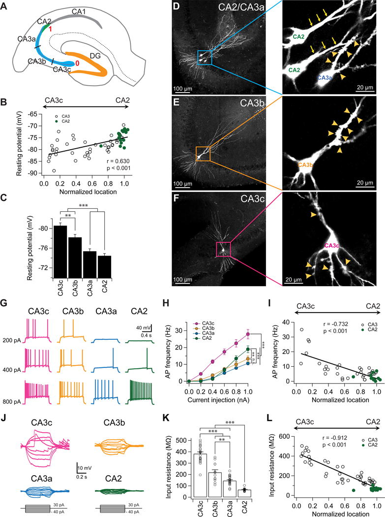
(A) Schematic diagram of a transverse hippocampal slice. CA3 is divided into three equal-sized regions along the transverse axis (CA3c, CA3b, and CA3a). The location of each recorded neuron was normalized from 0 to 1 based on their transverse location. PNs located at the beginning of the mossy fibers near DG were assigned a location of “0”, whereas neurons located at the end of the mossy fibers near CA2 were assigned a location of “1”.

(B) Resting membrane potential plotted against normalized cell location.

(C) Mean resting membrane potential in indicated subregions. Error bars show SE. **p < 0.01, ***p < 0.001. n = 16–32 neurons per group.

(D) Sample images of CA2 and CA3a PNs filled with biocytin. Note the absence (CA2, arrows) and presence (CA3a, arrowheads) of thorny excrescences in the expanded view (right).

(E) Sample images of a CA3b PN filled with biocytin. Note the presence of thorny excrescences (arrowheads) in the expanded view (right).

(F) Sample images of a CA3c PN filled with biocytin. Note the presence of thorny excrescences (arrowheads) in both basal and apical dendrites in the expanded view (right).

(G) Sample traces of firing patterns in response to indicated constant current injection.

(H) Mean firing frequency during the current step as function of current injection. Error bars show SE. **p < 0.01, ***p < 0.001. n = 15–24 neurons per group.

(I) AP frequency in response to a 1 s, 600 pA current injection plotted against normalized cell location.

(J) Sample traces of subthreshold membrane voltage responses to indicated current injections.

(K) Mean input resistance in indicated subregions. Error bars show SE. **p < 0.01, ***p < 0.001. n = 12–20 neurons per group.

(L) Input resistance plotted against the normalized cell location.