Figure 1.

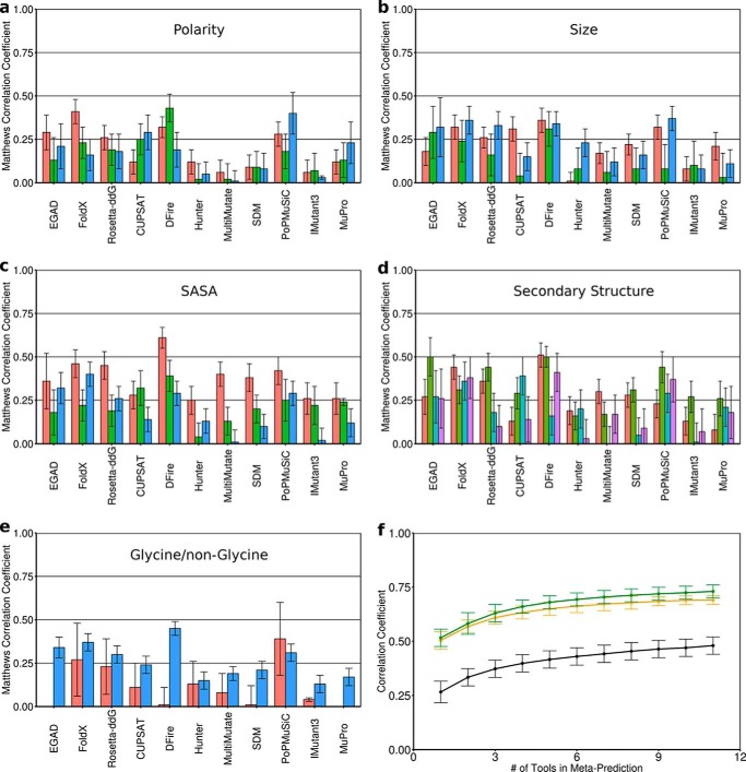
Building the meta-predictor. The performance of each tool as measured by MCC (96) is shown for different classifications of point mutations. a, polarity: decreased (red), similar (green), increased (blue). b, size: smaller (red), similar (green), larger (blue). c, solvent-accessible surface area of the WT residue: buried (red), partially exposed (green), exposed (blue). d, secondary structure of the backbone at the mutated position: helical (red), strand (green), turn (cyan), unstructured (purple). e, whether the mutation is to/from a glycine (red) or non-glycine (cyan). f, the more tools that were combined in the meta-predictor, the better the average performance, shown for MCC (black), ρ (orange), and R (green). Error bars (a–e), S.D. from 1000 analyses using 50% of the mutation data set. Individual predictors are grouped based on methodology: physical force field (EGAD), empirical potentials (FoldX and Rosetta), statistical potentials without machine learning (CUPSAT, DFire, Hunter, MultiMutate, and SDM), statistical potentials with machine learning (PoPMuSiC), and feature-based with machine learning (IMutant3 and MuPro).