Figure - PMC

Skip to main content

An official website of the United States government

Here's how you know

Here's how you know

Official websites use .gov
A .gov website belongs to an official government organization in the United States.

Secure .gov websites use HTTPS
A lock ( ) or https:// means you've safely connected to the .gov website. Share sensitive information only on official, secure websites.

View full-text article in PMC

. 2017 Sep 4;216(9):2911–2926. doi: 10.1083/jcb.201605119

Search in PMC
Search in PubMed
View in NLM Catalog
Add to search

© 2017 Capurro et al.

This article is distributed under the terms of an Attribution–Noncommercial–Share Alike–No Mirror Sites license for the first six months after the publication date (see http://www.rupress.org/terms/). After six months it is available under a Creative Commons License (Attribution–Noncommercial–Share Alike 4.0 International license, as described at https://creativecommons.org/licenses/by-nc-sa/4.0/).

PMC Copyright notice

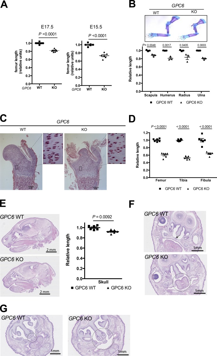
Figure 2. — GPC6-null mice display shorter long bones and face dysmorphisms. (A) Whole femurs were dissected from E17.5 or E15.5 embryos of the indicated genotypes. Images were acquired with a camera (DFC 295; Leica) using a stereoscope (M60; Leica), and femur length was measured using the Leica Application Suite (V3.8). Scatter plots with the mean ± SEM of eight WT and seven KO embryos are shown. Mean WT femur length in each litter was arbitrarily assigned the value of 1. (B, top) Upper limbs were dissected from GPC6 WT and GPC6 KO E18.5 embryos and stained with Alcian blue–Alizarin red. Images were acquired with a camera (DFC 295) using a stereoscope (M60). Representative bones are shown. (Bottom) Images from three WT and three KO femurs from different litters were measured with the Leica Application Suite (V3.8). The graph shows scatter plots with the mean ± SEM. (C) Proximal femoral metaphysis from E17.5 embryos of the indicated genotypes were stained with hematoxylin/eosin, and pictures were taken under the microscope. Insets represent an eight-times enlargement of the low-power picture. Bars, 100 µm. (D) The indicated bones were dissected from GPC6 WT (n = 6) and GPC6 KO (n = 6) E18.5 embryos and stained with Alcian blue–Alizarin red. Images were acquired, and the lengths of the diaphysis were measured as in B. The graph show scatter plots with the mean ± SEM. Mean WT bone length in each litter was arbitrarily assigned the value of 1. (E, left) Representative sagittal head sections corresponding to E18.5 GPC6 WT and GPC6 KO embryos. (Right) Skull length from the base of the skull to the end of nasal plenum was measured in GPC6 WT (n = 6) and KO (n = 6) embryos. Results are shown as a scatter plot with the mean ± SEM. Mean WT skull length in each litter was arbitrarily assigned the value of 1. (F and G) Representative cross-sections of the skulls of E18.5 embryos of the indicated genotypes illustrating the palatoschisis (arrow and circle; F) and nasal septal aplasia (circles; G) observed in the GPC6-null mice with a 100% penetrance (n = 5 of each genotype). Statistical analysis was performed by Student’s t tests (unpaired two-tailed).