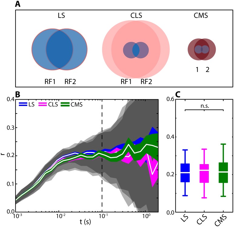
Fig 7. Experimentally measured differences in RF structure across the ELL maps give rise to similar levels of correlation in our model.

(A) RF organization for our model LS, CLS and CMS neurons. These are based on previously published experimental data [28] and our numerical simulations. The impact of RF surround on correlations was small in LS (size relation = 1:0.065; gain relation = 1:1.47), moderate in CLS (size = 1:12; gain = 1:0.4), and strong in CMS (size = 1:6; gain = 1:12). (B) Spike-count correlations for LS (blue), CLS (magenta) and CMS (green) as a function of time window corresponding to the RF structures shown in (A). Shown are mean (white lines), SEM (colored areas) and STD (gray shaded areas) correlation coefficients calculated across 50 realizations of the model. The correlation coefficients predicted for the three segments were similar and thus largely overlapped with one another. (at T = 100 ms: median LS: 0.24, range: -0.44–0.79; CLS: 0.24, -0.57–0.67; CMS: 0.26, -0.20–0.71). (C) Distribution of correlation coefficients calculated for t = 100 ms (see vertical dotted line in B). At this timescale, the means of the distributions were not significantly different from one another (Kruskal-Wallis; dF = 2; Chi² = 1.8; p = 0.41). Qualitatively similar results were obtained for other time windows (e.g.: t = 10 ms; Chi² = 4.27; p = 0.12; or t = 1 s; Chi² = 1.23; p = 0.54).