Fig. 5.

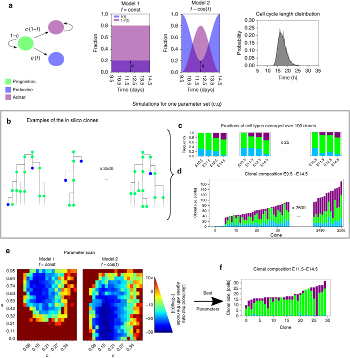
Stochastic model of clonal expansion. a Probabilistic transitions among three states are presented in a state diagram: at the division progenitors (green) differentiate with probability c and maintain progentor state with probability 1 − c. When differentiating, they become endocrine (blue) with probability f and acinar (purple) with probability 1 − f. We compare two models: in Model 1 the probability f is constant between E9.5 and E14.5, and in Model 2f is time-dependent and has a minmum at around E12. The height of the minimum is characterised by parameter q. In Model 1 f = g. See Methods for the exact functional form of f for Model 2. While acinar cells continue replicating, endocrine cells are assumed not to replicate. For all replicating cells the cell-cycle lengths are drawn from the gamma distribtuion from¹⁹ (right panel). For every parameter set both models were simulated 2500 times. b Examples of the in silico clonal lineages. c Fraction of cell types from individual clones at E9.5, 11.5, 12.5 and 14.5 (corresponds to experimental data in Supplementary Fig. 7d). d Clonal composition at E14.5 (corresponds to Figs. 1h and 4f). e For each of the parameter sets c, q we estimate the likelihood of the model fitting the data (See Methods and Supplementary Figs. 8–10). The results of the parameter scan are quantified by the log-likelihood, −2log(L). Parameter scans show that Model 2, where the differention of acinar cells and endocrine cells change with time, is more likely. Using Akaike Information Criteria score, AIC, we find that Model 2 is better at describing the data (AIC₁ = −14.5 and AIC₂ = −22.1). The probability that the two models are equally good is p = 0.02. f The model predicts that if clonal anlyses are started at E11.5–12 instead of E9.5, it becomes more likely to observe lineages fully commiting to the acinar fate