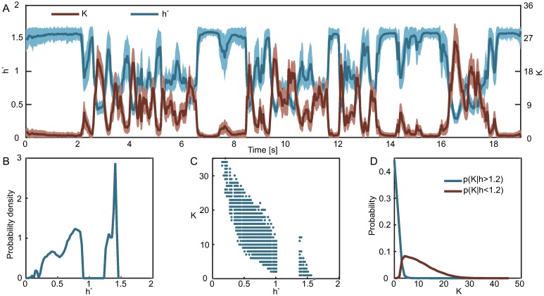
Fig 7. The most likely value of the latent variable naturally defines two global population states.

A) For every repeat of the stimulus and for every time bin we estimate the most likely value of the latent (h*) given the population response at that time, as well as the total number of spiking neurons in that response (K). The plot shows the trajectories of h* and K averaged across repeats. Error bars correspond to 1 SD. B) Probability density of h*, i.e. the most likely value of the latent given the population response. C) A scatter plot of the total network activity vs. the most likely value of the latent. h* naturally divides the population responses into two clusters. D) Probability distribution of the total network activity given this global population state. While the most likely value of K for low h* is zero, the distribution has a tail that extends to K ≈ 5.