A latent low-dimensional common input drives a pool of motor neurons: a probabilistic latent state-space model

We propose a state-space model that explicitly delineates a common input signal sent to motor neurons and the physiological noise inherent in synaptic signal transmission. This is the first application of a deterministic state-space model to represent the discharge characteristics of motor units during voluntary contractions.

Abstract

Motor neurons appear to be activated with a common input signal that modulates the discharge activity of all neurons in the motor nucleus. It has proven difficult for neurophysiologists to quantify the variability in a common input signal, but characterization of such a signal may improve our understanding of how the activation signal varies across motor tasks. Contemporary methods of quantifying the common input to motor neurons rely on compiling discrete action potentials into continuous time series, assuming the motor pool acts as a linear filter, and requiring signals to be of sufficient duration for frequency analysis. We introduce a space-state model in which the discharge activity of motor neurons is modeled as inhomogeneous Poisson processes and propose a method to quantify an abstract latent trajectory that represents the common input received by motor neurons. The approach also approximates the variation in synaptic noise in the common input signal. The model is validated with four data sets: a simulation of 120 motor units, a pair of integrate-and-fire neurons with a Renshaw cell providing inhibitory feedback, the discharge activity of 10 integrate-and-fire neurons, and the discharge times of concurrently active motor units during an isometric voluntary contraction. The simulations revealed that a latent state-space model is able to quantify the trajectory and variability of the common input signal across all four conditions. When compared with the cumulative spike train method of characterizing common input, the state-space approach was more sensitive to the details of the common input current and was less influenced by the duration of the signal. The state-space approach appears to be capable of detecting rather modest changes in common input signals across conditions.

NEW & NOTEWORTHY We propose a state-space model that explicitly delineates a common input signal sent to motor neurons and the physiological noise inherent in synaptic signal transmission. This is the first application of a deterministic state-space model to represent the discharge characteristics of motor units during voluntary contractions.

when adrian and bronk (1929) first recorded motor unit action potentials in humans, they hypothesized that a common presynaptic signal could underlie the control of motor neuron discharge characteristics. Initial attempts to characterize the common input signal focused on quantifying the correlated activity between pairs of motor units (Sears and Stagg 1976). However, the magnitude of the pairwise correlations has generally been found to be weak and variable (Bremner et al. 1991; De Luca et al. 1982, De Luca and Erim 1994; Farmer et al. 1993; Nordstrom et al. 1992), suggesting that such comparisons cannot be used to quantify common input (Farina and Negro 2015). An alternative approach is to record the discharge times of at least five concurrently active motor units and to assume that the motor unit pool acts as a linear filter of the independent synaptic noise delivered to motor neurons, which produces an output that corresponds to the neural drive to the muscle (Farina et al. 2014; Farina and Negro 2015; Negro et al. 2009, 2016a). As an extension of this approach, Boonstra et al. (2016) proposed an explicit biophysical model to represent the effect of the common synaptic input onto the motor neurons. Each neuron was represented as an integrate-and-fire neuron that filtered the weighted synaptic inputs to allow more realistic connection topology and enable a structural definition of common input.

However, these approaches have mathematical and methodological limitations. One principal objection is that action potentials are discrete events and should be represented as point processes rather than continuous-time stochastic processes (Buesing et al. 2012; Macke et al. 2011, 2015). The computation of second-order statistics, such as coherence (e.g., De Luca et al. 1982, De Luca and Erim 1994; Sears and Stagg 1976) or principal component analysis (Negro et al. 2009), is not adapted to point processes (Kuhn et al. 2003). Additionally, contemporary approaches rely on the motor unit pool acting as a linear filter of the synaptic input, whereas some properties of the motor pool, such as persistent inward currents, make the motor unit pool highly nonlinear (Powers and Heckman 2017). Moreover, failure to account for distinct sources of input to the motor neuron pool (Boonstra et al. 2016) means that the same second-order statistics could be produced by quite different physiological mechanisms.

In contrast, state-space models explicitly describe the interactions between neurons and the influence of common input. Such probabilistic models are uniquely characterized by a few parameters that can be estimated from the discharge times of activated neurons. The models are able to decode neuronal connectivity, the common input, and their associated statistical significances. These models have been used successfully to analyze spike trains of neuronal data recorded in the central nervous system (Ahmadian et al. 2011; Dempster et al. 1977; Paninski et al. 2010; Pnevmatikakis et al. 2016; Truccolo 2010). Moreover, present approaches require a sufficiently long signal to create a cumulative spike train that is amenable to frequency analysis. A state-space model, in contrast, can be used to examine relatively brief isometric contractions. The current study analyzes, for the first time, the activity within an entire motor unit population with a state-space model. The proposed model expresses the common modulatory input as an unobserved (latent) state vector that varies in time to generate a net muscle force that matches a target force. The latent common input is perturbed by random synaptic noise. The temporal variation exhibited by the latent state, which encodes the synaptic input common to the motor neuron pool, can be interpreted as an abstract trajectory.

State-space models seek to explain the activity of many outputs through an n-dimensional vector referred to as the latent state of the system. The latent state changes over time with an abstract magnitude, where the absolute value at any one time need not be physiologically meaningful, but the trajectory of the latent state provides insight on the overall dynamics of the common input received by the motor neurons. Additionally, the variance in the latent-state trajectory may approximate the synaptic noise that is common to all motor units. More generally, the common input estimated by the state-space model could be used to assess the influence of other confounding factors, such as adjustments during fatiguing contractions or age-related differences.

The key idea of the present study was to represent the discharge activity of each motor neuron using an individual Poisson process (Berg et al. 2008; Perkel et al. 1967; Person 1974; Person and Kudina 1972; Powers et al. 2005; Townsend et al. 2006); the parameters of the proposed model are relatively insensitive to the distribution characteristics of the motor unit interspike intervals. The rate (intensity) of the Poisson process is modulated by the latent common input and the activity of the other neurons in the pool. The discharge times of each motor unit are represented as a Poisson point process that can be sampled at a high rate and evaluated with fast algorithms that have already been developed (Buesing et al. 2012; Macke et al. 2011). The parameters of the model and the common input can be estimated from the discharge times of the motor neurons (Mangion et al. 2011; Smith and Brown 2003).

The dimensionality of the latent common input can also be estimated using a goodness-of-fit criterion (Macke et al. 2015). Once the parameters have been estimated, the model allows for explicit quantification of the trajectory of the common input signal and, separately, a synaptic noise term. Macke et al. (2015) note that dynamic state-space models provide a good fit for discharge times for two reasons. First, they can accommodate data for many neurons at fine time scales, which reduces the likelihood that shared variability is coincidental. Second, this class of models naturally captures the almost instantaneous (time lag ∼0) peak in cross-correlation of motor unit discharge rates (De Luca et al 1982, De Luca and Erim 1994) through a latent state trajectory (Macke et al. 2015).

The purpose of the present study was to estimate the synaptic input and its associated variance that is common to a pool of motor neurons. The model was derived from state-space models that have been used to decode the influence of sensory pathways on activity exhibited by cortical neurons (Macke et al. 2011) and spinal cord neurons (Buesing et al. 2012). This approach is validated with four different data sets: the replication of experimentally observed motor unit discharge characteristics; the discharge times for a pair of integrate-and-fire neurons, with a Renshaw cell providing negative feedback; the discharge activity of 10 integrate-and-fire neurons, which is compared with the contemporary approach to assess common input; and quantification of the common input to motor neurons derived from an experimental recording of motor unit discharge rates.

METHODS

The mathematical model comprises a low-dimensional common input to a pool of motor neurons to represent a common input signal and a synaptic noise term explicitly. This work advances previous models of motor unit recruitment (Dideriksen et al. 2010; Fuglevand et al. 1993; Moritz et al. 2005) and is based on work performed on the statistical structure of neuronal discharge times in the motor cortex (Macke et al. 2011) and sensory pathways (Archer et al. 2014). Although some previous models of motor unit recruitment model the presynaptic input to a motor unit pool (Watanabe et al. 2013; Williams and Baker 2009), most do not (Fuglevand et al. 1993; Moritz et al. 2005). The present work provides a model based on a dynamical system, which can be fit to experimental recordings of motor units for the purpose of quantifying the common input to the motor neuron pool.

An overview of the proposed model is shown in Fig. 1. This model utilizes the discharge rate λ_i(t) to represent the nonlinearity between an input current and the discharge times of a neuron, i. The discharge times y_i(t) of each motor unit (i = 1…n) are parameterized as a Poisson point processs, where the time-varying intensity (discharge rate), λ_i(t), of the ith motor neuron takes the following form:

Fig. 1.

The state-space model represents the processes that are engaged to enable a population of motor units to produce a force that matches a desired target force. The trajectory of the latent state, X(t), must evolve to provide sufficient activation to the pool of motor neurons for them to discharge action potentials. The changes in the latent state over time are captured by the matrix, A, which represents a linear approximation of the latent-state dynamics. All neurons receive two inputs, a common input (the latent state) that excites the motor neurons and zero-mean Gaussian synaptic noise. The physiological properties of each neuron are modeled with the C matrix, which encodes the effects of the input signal on discharge rate. The output is instantaneous discharge rates of each motor neuron, which evolve as the latent state changes. The forces generated by the activated motor units are summed to create the net muscle force.

$${\lambda }_i\left(t\right)=\exp \left[{\text{z}}_i\left(t\right)\right]\mathrm{.}$$ 1)

The exponential relation ensures that the rates are positive and explicitly encodes the influence of a latent, low-dimensional common input through the n-dimensional vector z (t) = $\left[{\text{z}}_1\left(t\right),\mathrm{..},{\text{z}}_{\text{n}}\left(t\right)\right]$ in the following linear model:

$$z\left(t\right)=Cx\left(t\right)+Ds\left(t\right)+\mu \mathrm{.}$$ 2)

where x(t) is a d-dimensional vector that represents the unobserved common input, C is an n × d matrix that encodes the physiological effects of the latent common input on the motor discharge rates, D is an n × n matrix that models the coupling between the n motor units, s may be defined to model the interconnectivity of motor neurons, and μ is the logarithm of the average discharge rate, which provides a baseline discharge rate (variables in boldface represent matrices or vectors; non-boldface variables represent scalar values). Additionally, s(t) may be conditioned by the previous discharge activity of the motor units (Buesing et al. 2012; Macke et al. 2011, 2015), which allows for feedback to be modeled from a motor neuron to itself as well as the other neurons in the network. For example, an inhibitory input between neurons could be modeled with a value between 0 and 1 on the corresponding entry in s(t) between the neurons, whereas an excitatory input would be modeled with an entry >1. With this approach, s(t) allows for modulation of discharge rate by excitatory and inhibitory inputs.

The common input is expected to vary as a function of time and target force. The dynamics of the common input is described as follows:

$$x\left(t\right)=Ax\left(t-1\right)+b\text{f}\left(t\right)+\epsilon \left(t\right),$$ 3)

where A is an n × n matrix that provides a linear approximation to the dynamics of the n motor units, the n-dimensional vector b weights the influence of the force target f(t) on each coordinate of x(t), and the Gaussian vector ε(t) is the zero mean Gaussian noise vector that models the synaptic noise inherent in signal transmission, such as the opening and closing of ion channels (Katz and Miledi 1970).

In this model, x(t) represents the low-dimensional approximation to the latent state that activates a pool of motor neurons, which is often described as the common input. Following Macke et al. (2011), we assume that the common input evolves according to linear Gaussian dynamics, which depends on the intended target force bf(t) according to the following probability distributions:

$$x_1~\mathcal{N}\left(x_o,Q_o\right),$$

$$x_t|x_{t-1}~\mathcal{N}\left(A{x}_{t-1}+b{\text{f}}_t,Q\right),$$ 4)

where x₀ and Q₀ represent the initial state and covariance matrix, respectively, of the latent input x_t, and Q is a covariance matrix of the latent state x_t and represents the physiological random fluctuations in the common input signal. We further assume that Q remains constant over time.

Motor unit model.

The first experiment demonstrated the ability of the model to recover the parameters of a synthetic data set generated by modeling ramp contractions of a pool of 120 motor units in the first dorsal interosseus muscle (Feinstein et al. 1955). The model was based on the original Fuglevand model (Fuglevand et al. 1993). Simulations were performed 10 times at each target force [from 5 to 30% maximal voluntary contraction (MVC)]. Each trial involved an excitatory drive function that comprised a linear 1-s ramp from 0 N to the target force (%MVC) that was maintained for 4 s. Each motor neuron received a common input signal and a noise signal inversely proportional to the difference between its recruitment threshold force and the target force. The recruitment threshold excitation (RTE) for the ith motor unit was set to

$$RTE(i)=e^{a\times i},$$ 5)

where a establishes an exponential range of threshold values based on the upper limit of motor unit recruitment a = (1n60)/120, where 60 refers to 60% MVC force and represents the upper limit of motor unit recruitment (Dideriksen et al. 2010; Moritz et al. 2005), and n = 120 denotes the number of motor units in the model. Motor units were recruited during the ramp contraction once the level of excitation exceeded RTE. The resulting discharge rate was determined by the evolution of the latent state and the physiological parameters of the motor unit pool. In these simulations, the common input was approximated with a one-dimensional latent input that activates the pool of motor neurons to reach the target force in 1 s and maintain it for 4 s.

The matrix C was modeled as a 1 × n matrix, where n represented the number of active units. Each row of C represented the response of a motor neuron to the latent input. The 120 units were assigned to respond to the latent input so that the minimal discharge rate for the first recruited motor unit was between 6 and 8 pps. The column in C was derived to represent the range of physiological parameters within a motor pool that would influence discharge rate, such as the fivefold range in afterhyperpolarization duration and 10-fold range in input conductance (Heckman and Enoka 2012). The magnitude of each row was estimated to produce realistic discharge rates and thereby demonstrate the feasibility of the algorithm. The following linear function determined the values of C:

$$C_i=2+0.0054\times i\mathrm{.}$$ 6)

The evolution of the latent state during the 5-s simulations was modeled by Eq. 3. After the target force was reached (1-s ramp), the force term bf(t) was held constant. The synaptic noise ε(t) received by each motor neuron was modeled by a zero-mean white Gaussian noise and was added to the signal using awgn in MATLAB. This noise was proportional to the difference between RTE for the ith unit and the present level of excitation. The plateau in discharge rate (saturation) observed in low-threshold motor units (Bigland and Lippold 1954; Fuglevand et al. 2015; Monster and Chan 1977; Moritz et al. 2005; Barry et al. 2007), captured by the vector b in Eq. 3, was modeled using a hyperbolic tangent function:

$${\text{b}}_i=\frac{1}{2}\left\{\tanh \left[\text{ARTE}\left(i\right)\right]+1\right\},$$ 7)

where ARTE was the difference between RTE for the ith motor unit and the force (%MVC) at any time t, which represented the current level of excitation being received by the motor neurons. Based on this relation, the difference between the level of excitation and the recruitment threshold force influenced motor unit discharge rate through b. The discharge rate λ_i(t) of each neuron i was updated every 10 ms according to the following equation:

$$\text{exp}\left\{{\left[C\left(Ax\left(t\right)+bf\left(t\right)+\epsilon \right)\right]}_i\right\}\mathrm{.}$$ 8)

Force model.

The force produced by each motor unit in response to an action potential was modeled as a critically damped second-order system (Fuglevand et al. 1993; Milner-Brown et al. 1973). As defined in the Fuglevand model, the twitch force, f_i(t), for the ith motor unit was determined as

$$f_i(t)=\frac{P_i\times \text{t}}{T_i}\times e^{1-\left(\frac{t}{Ti}\right)},$$ 9)

where P represents the twitch force and T denotes the twitch contraction time for each of the n motor units. Peak twitch force for the 120 motor units was assigned with an exponential function that established a 100-fold range of twitch forces (Fuglevand et al. 1993):

$$P(i)=e^{b\times i}=e^{\frac{\text{ln}\left(100\right)}{120}\times i}\mathrm{.}$$ 10)

The twitch contraction times varied with peak twitch force so that units with the greatest peak twitch forces also had the fastest twitch contraction times (Fuglevand et al. 1993). Twitch contraction times were scaled to exhibit a threefold range:

$$\text{T}(i)=90\times {\left(\frac{1}{Pi}\right)}^{1/4.2}\mathrm{.}$$ 11)

The nonlinearity between stimulus frequency and motor unit force (Fuglevand et al. 1993; Kernell and Monster 1981; Milner-Brown et al. 1973) was modeled with a sigmoid gain that augmented force for brief adjacent interspike intervals. Specifically, the normalized discharge rate for the ith unit with an interspike interval (ISI) at time t, (T_i/ISI_t) summed twitch forces with the following gain:

$$S\left(\frac{T_i}{ISI}\right)=1-e^{-2{\left(\frac{Ti}{ISI}\right)}^3}\mathrm{.}$$ 12)

Normalized discharge rate was defined as the contraction time for the ith motor unit divided by the interspike interval between t and t − 1. The gain was defined with a piecewise function for each unit at time t. The sigmoidal gain was expressed as the ratio of the gain divided by the instantaneous normalized discharge rate for rates ≥0.4. At normalized discharge rates <0.4, motor unit forces were not scaled with a gain. Overall, the gain was defined by

$$Gain=\{\begin{array}{c}\hspace{0.17em}\frac{S\left(\frac{Ti}{ISI}\right)}{\frac{Ti}{\text{ISI}}}if\frac{T_i}{ISI}\ge 0.4\hspace{0.17em}\\ 0\hspace{0.17em}\hspace{0.17em}otherwise\end{array}\mathrm{.}$$ 13)

The net force produced by the motor unit pool was calculated as the instantaneous sum of the ith motor unit force at time j updated at a rate of 10 Hz:

$$\sum _{i=1}^k{f}_{i,j}\hspace{0.17em}=\hspace{0.17em}f\left(t-t_{i,j}\right)\mathrm{.}$$ 14)

The force model was developed in MATLAB (Version 2015a; The MathWorks, Natick, MA) and run 10 times at four target forces: 5, 10, 20, and 30% MVC. The outputs of the model were instantaneous discharge rates for the pool of motor units. Random realizations of an inhomogeneous Poisson process were generated using the intensity λ_i(t) (using the MATLAB function exprnd). The variables of interest were the average discharge rates for the motor units during the steady portion of the contraction, the variability in discharge times (interspike intervals), the mean force and its variability, and the spectral content of the force signal.

Integrate-and-fire neuron models.

The model was used to simulate the discharge times of action potentials for a pair of integrate-and-fire neurons, with a Renshaw cell providing negative feedback from one neuron to the other one (Kirkwood et al. 1981; Windhorst 1989). The purpose of the simulation was to demonstrate that the state-space model is able to quantify neural pathways with inhibitory and excitatory feedback loops. Additionally, the simulation provided an intuitive understanding of the characteristics of a latent-state trajectory in that there was a change in the magnitude of the latent state when the neurons discharged action potentials. Both neurons were simulated with a capacitance of 1 nF, a resistance of 40 mΩ, a resting membrane potential of −65 mV, and a voltage threshold of −55 mV. A sinusoidal input current (1 nA) was delivered to both neurons at 3 Hz. A recurrent collateral from neuron A projected to a Renshaw cell (C), which synapsed onto neuron B and elicited an inhibitory postsynaptic potential of 1 mV decaying to 0 mV over 10 ms after each action potential discharged by neuron B. The currents received on the soma of the neurons were integrated using Euler’s method updating every 1 ms. Figure 2 provides an overview of the model for a pair of integrate-and-fire neurons.

Fig. 2.

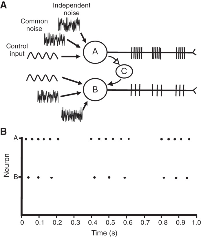
Schematic for a pair of motor neurons, with a collateral from neuron A projecting to a Renshaw cell (C) that then elicited inhibitory postsynaptic potentials in the 2nd motor neuron (neuron B). The solid arrow projecting to neuron B indicates an inhibitory projection. A: schematic overview of the leaky integrate-and-fire neurons (neurons A and B) with an interposed Renshaw. Motor neurons (neurons A and B) received 3 inputs: control signal, common noise, and independent noise. B: Raster plot of the discharge times for action potentials from motor neurons A and B.

Each neuron received three inputs concurrently: a sinusoidal common input, zero mean Gaussian common noise, and zero mean Gaussian-independent noise. When the potential difference across the membrane reached voltage threshold (−55 mV), the neuron discharged an action potential with an overshoot that reached +10 mV, followed by an afterhyperpolarization phase where the potential difference dropped to −70 mV and rose to −65 mV linearly over the course of 50 ms. The discharge times of the two motor neurons (neurons A and B) were summed at each instant to form a cumulative spike train (CST), which was subsequently low-pass filtered (6th-order Butterworth filter, cutoff frequency 10 Hz) (Castronovo et al. 2015; Farina et al. 2014; Negro et al. 2016a). The filtered CST represents one method to represent the common input to the motor neurons. The coherence between the filtered CST and the input current was calculated with Welch’s periodogram method in MATLAB using the function “mscohere” with a 90% overlap and a 0.25-s Hanning window. Additionally, the latent vector, x(t) and its corresponding covariance matrix were optimally estimated using an expectation maximization (EM) algorithm (Buesing et al. 2012; Macke et al. 2011). The integrate-and-fire neurons were simulated for two durations (1 and 10 s) to demonstrate the capacity of a state-space model to estimate common input for relatively brief signals for which frequency analysis is less robust.

A set of 10 integrate-and-fire neurons were simulated for two input frequencies (3 and 4 Hz) and three current amplitudes (0.1, 0.5, and 1 nA). The neurons were simulated with a range of input resistances linearly spaced from 35 to 80 mΩ and capacitance from 0.9 to 1.8 nF. All neurons received two inputs: the control input (either 3 or 4 Hz) and a common noise using the awgn function in MATLAB with a signal-to-noise ratio of 25. All simulations were performed for 10 s. Cumulative spike trains (CSTs) were constructed (Castronovo et al. 2015; Farina et al. 2014; Negro et al. 2016a) and low-pass filtered. The spectral content of the CST was calculated with a Fast Fourier transform (FFT; MATLAB). Additionally, the discharge times from the 10 integrate-and-fire neurons were used to estimate the parameters of the state-space model using PLDS example (Macke et al. 2015). The number of neurons included in the simulations was set at 10 to match the number of concurrently active motor units that can be discriminated from high-density surface EMG recordings during submaximal voluntary contractions.

The code for these simulations is available at github.com/dfeeney31 within the neural model repository.

Experimental procedures.

The IRB at the University of Colorado Boulder approved this study (approval no. 16-0782). A single subject performed isometric contractions at 10% MVC force with the elbow flexor muscles. High-density grid electrodes (64 mm, 8-mm interelectrode distance; Bioelettronica, Torino, Italy) were placed over the long head of the biceps brachii muscle. The EMG signals from the grid electrodes were recorded at 2048 Hz and decomposed using a semiautomated convolution kernel algorithm implemented in MATLAB (Holobar and Zazula 2004; Negro et al. 2016b). The discharge times for seven motor units were identified during the trial. The motor unit discharge times were arranged into an nxT binary discharge matrix, with each row representing a motor unit at T time samples during the last 20 s of the isometric contraction. The matrix of motor unit discharge times was down sampled to bin widths of 10 ms for purposes of estimating the parameters of the state-space model. The parameters of the state-space model [specifically x(t) and Q] were estimated using an EM algorithm (Buesing et al. 2012; Macke et al. 2011). Coherence was calculated between the trajectory of single dimensional latent state and the net elbow flexor force. The trajectory and variance of the latent state estimate of the common input received by the motor neurons were estimated during the last 20 s of the contraction. Welch’s averaged modified periodogram was used to calculate the coherence between the input current (or the force signal) and the trajectory of the latent state using the function mscohere in MATLAB with a 90% overlapping window and a Hanning window of 0.5 s as suggested in Castronovo et al. (2015). The 95% confidence intervals of the coherence were determined using the function cmtm in MATLAB.

Estimating model parameters.

An open-source expectation maximization (EM) algorithm (PLDSExampleWithExternalInput from the pop_spike_dyn directory on Atlassian BitBucket; Macke et al. 2011) was used to estimate the parameters of the proposed state-space model for the simulations and experimental data. A Poisson subspace identification method was used for all estimations, which has been shown to be the most accurate for neural data and is described in detail by Buesing et al. (2012). Briefly, the input to the algorithm was a matrix of the motor unit discharge times that were used to estimate the trajectory of the latent state and to quantify the variability in its trajectory (Buesing et al. 2012; Macke et al. 2015). The parameters of the model were initialized using a Poisson subspace initialization (Buesing et al. 2012). Subsequently, a Ho-Kalman filter state space identification algorithm (Ho and Kalman 1966) was used to estimate the parameters of the state-space model iteratively. The maximal log likelihood of the posterior distribution of the latent vector (x(t)) was used to determine the goodness of fit of the model. The EM algorithm iteratively refined the initial estimation until a local maximum of the log-likelihood function had been reached. The EM algorithm was stopped when either a maximum number of iterations (100) was reached or when the relative error in log likelihood became smaller than 10⁻³.

In principle, the estimation of the latent space model can be performed for a latent-space vector of varying complexity by changing the dimension of that vector. To prevent over-fitting, however, the dimensionality of the latent state was chosen to be the lowest dimension after which the log-likelihood no longer increased (Macke et al. 2011). Additionally, any dimension for which the estimated variance was numerically negligible was removed. Consequently, the dimension of the latent space was the lowest dimension that resulted in the maximum of the estimated log likelihood while keeping the variance of all coordinates greater than a threshold chosen to be 10⁻⁴.

State-space models assume the variance in the input signal is constant (stationary) during a particular task. However, nonstationary input to motor neurons, such as during long-lasting isometric contractions, can be examined by dividing the recording into segments in which the estimated parameters are relatively stationary. With this approach, it is possible to estimate how the latent input changes during long-lasting isometric contractions.

RESULTS

The results comprise predicted discharge rates of the motor neuron pool and the force fluctuations during a ramp-and-hold contraction. The discharge characteristics and force fluctuations of the model were compared with experimental findings for the first dorsal interosseus muscle.

Motor neuron discharge characteristics.

Table 1 lists the recruitment thresholds and the minimal and maximal discharge rates for every 10th motor unit in the simulated pool of units. As specified by Eq. 2, minimal and maximal discharge rates increased with recruitment threshold force. Minimal discharge rates ranged from 7.5 to 17.3 pps, and maximal discharge rates ranged from 13.2 to 30.2 pps. The data are similar to minimal (7–12 pps) and maximal (30 pps) discharge rates reported by Moritz et al. (2005) during steady isometric contractions with the first dorsal interosseus muscle. Coefficient of variation for the interspike interval for motor units ranged from 12.4 to 19.8% during the last 2 s of each contraction, which is slightly less than the 15 to 35% reported by Moritz et al. (2005).

Table 1.

Motor unit discharge characteristics obtained from the state-space model activating 120 simulated motor units

Motor Unit, no.	Minimum DR	Maximum DR	Recruitment Threshold, %MVC
10	7.5	13.2	1.4
20	7.8	14.5	2
30	8.3	15.4	2.8
40	9	16.8	3.9
50	9.8	17.5	5.5
60	10.8	18.3	7.7
70	12	20.1	10.9
80	13.3	21.2	15.3
90	14.8	23.2	21.6
100	16.5	24.5	30.3
110	16.8	26.9	42.7
120	17.3	30.2	60

DR, discharge rate; MVC, maximal voluntary contraction. Minimal discharge rates were calculated by setting the target force equal to the recruitment threshold of each motor unit. Subsequently, the force was set to 100% MVC, and the maximal discharge rates for each motor unit were determined. Recruitment threshold was calculated by solving Eq. 5: RTE_i = e^{a × i}, where a = ln(60)/120 for each motor unit.

Figure 3 depicts the number of motor units recruited and their discharge rates during simulated contractions to target forces of 5–30% MVC. Data are similar to those reported by Moritz et al. (2005). The hyperbolic tangent function also modeled the saturation of discharge rates seen when low-threshold motor units are tracked during ramp contractions (Fuglevand et al. 2015; Moritz et al. 2005; Monster and Chan 1977). At the 5% target force, for example, the first motor unit discharged action potentials at a rate of 8.5 pps and the 47th motor unit at 7.3 pps. At the 30% target force, the first motor unit had reached its peak discharge rate of 13.2 pps and the 47th motor unit discharged action potentials at 16.4 pps. These discharge rates compare well with those for Moritz et al. (2005), where an early recruited unit (motor unit 2 in the first table in Moritz et al. 2005) exhibited an initial discharge rate of 6.8 pps and a peak discharge rate of 13.8 pps. Similarly, the motor unit recruited at 9.2% MVC force (motor unit 14 in the first table in Moritz et al. 2005) displayed an initial discharge rate of 6.8 pps and a peak discharge rate of 19.2 pps.

Fig. 3.

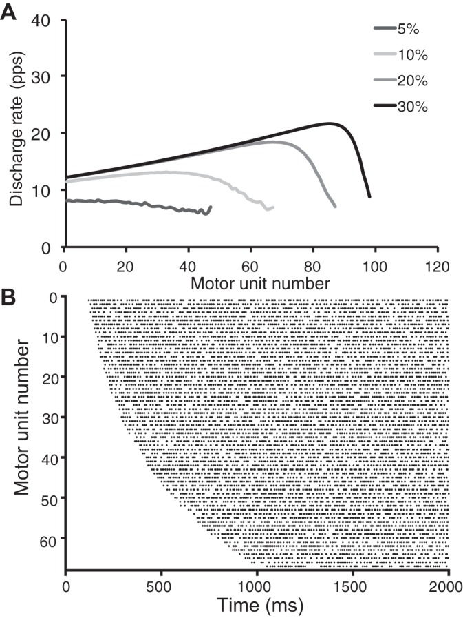
A: no. of motor units recruited and their discharge rates during simulated isometric contractions to match 4 target forces [5, 10, 20, and 30% maximal voluntary contraction (MVC)]. Average discharge rate was calculated from the last 2 s of each simulated contraction. B: Raster plot of the motor unit discharge times for the 67 motor units that were recruited during the first 2 s of a simulated 5-s contraction to a target force of 10% MVC. The task was comprised of a 1-s ramp and then a 4-s hold. The latent state activated the motor neurons to discharge action potentials as specified by the prescribed physiological properties. Each bin represents 10 ms.

Force model.

The discharge times of motor neurons were converted to motor unit forces as described in Eq. 15. The simulated muscle force at each target force is shown in Fig. 4A. The coefficient of variation of force during the hold phase (2–4 s) was greatest (5.9 ± 0.5%) for the simulated contraction at 5% MVC and least (2.1 ± 0.2%) for the simulated contraction at 30% MVC. The simulated values are compared in Fig. 4B with experimental measurements for first dorsal interosseus (Galganski et al. 1993; Moritz et al. 2005). Due to the low-pass filtering characteristics of muscle (Partridge 1965), 99% of the power in the force signal was in the low frequency (0–10 Hz) spectrum, which contains most of the spectral content important in force production during human movement (De Luca and Erim 1994; Farina and Negro 2015).

Fig. 4.

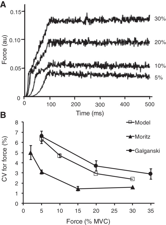
Simulated muscle forces during isometric contractions at 4 target forces. A: forces produced by the state-space model. The force fluctuations were quantified as the coefficient of variation for force during the last 2 s of each contraction. B: comparison of the simulated results obtained in the present study with experimental findings for the first dorsal interosseus muscle (Galganski et al. 1993; Moritz et al. 2005). Error bars represent the standard deviation.

Estimated parameters of the state-space model.

After the instantaneous discharge rates of motor neurons were converted into discharge times (see methods for explanation), the parameters of the state-space model at each target force were estimated using the EM algorithm described in methods. The discharge times of all motor neurons were arranged into a nxT matrix, where n is the number of active neurons during the trial and T is the number of time samples, using a resolution of 10 ms. Figure 5, A–D, shows the estimated latent-state trajectory in a single dimension during the 5-s trials at the four target forces (5, 10, 20, and 30% MVC). Both the ramp and steady portion of the trials were identified using the EM algorithm. Additionally, the variance in the single dimension of latent-state trajectory decreased with target force (0.0024 at 5% MVC compared with 0.0010 at 30% MVC). This decline in variance for the common input is consistent with the results reported by Castronovo et al. (2015), wherein the proportion of common input (relative to synaptic noise) was demonstrated to increase with net excitatory input.

Fig. 5.

Estimated trajectory of the single-dimensional latent state that activated the pool of neurons in the model as decoded by the expectation maximization (EM) algorithm (Macke et al. 2011). Estimated latent state trajectory at 5 (A), 10 (B), 20 (C), and 30% (D) MVC force. The magnitude and rate of change of the latent state trajectory specify the deterministic input to motor neurons. Higher resolution and corresponding calibration bar displayed last 2 s of trial at 5 and 30% MVC contractions.

Integrate-and-fire neurons.

The discharge of action potentials by the integrate-and-fire neurons was simulated for 1 s when they were provided with three currents: common input, common noise, and independent noise (Fig. 2A). The discharge times of the two motor neurons are displayed in Fig. 2B. Motor neuron A discharged action potentials at 13 pps and, due to the negative feedback from the Renshaw cell (C), the second motor neuron (neuron B) discharged action potentials at 9 pps, which represented a 30% decline in its discharge rate. The space-state vector was estimated from the discharge times of the two motor neurons with an EM algorithm (see methods). Critically, the latent-state trajectory aligned with the peaks in injected current to the pair of integrate-and-fire neurons (Fig. 6A), which demonstrates the feasibility of this model to identify the space-state parameters for groups of neurons with negative feedback from Renshaw cells. In contrast, the CST approach was unable to detect any difference in coherence below 10 Hz between the common input signal (at 3 Hz) and the low-pass-filtered CST when the simulation lasted only 1 s (Fig. 6B).

Fig. 6.

Estimation of the state-space model from a pair of integrate-and-fire neurons (see Fig. 2) simulated for 1 (A and B) and 10 s (C and D). Both neurons discharged action potentials in response to a 0.1-nA sinusoidal current with an input frequency of 3 Hz as well as receiving independent and common Gaussian noise. Additionally, neuron B received an inhibitory current from neuron C (a Renshaw cell) in response to input from neuron A, which reduced the discharge rate of neuron B. The trajectory of the single-dimension approximation of the latent state for the pair of neurons as solved with the EM algorithm is shown as a black solid line (Buesing et al. 2012; Macke et al. 2011), the injected current with common noise superimposed is drawn as a dashed line, and the low-pass-filtered (10 Hz) cumulative spike train (CST) is indicated as a gray line. There was a strong temporal relation between peaks in the injected current and changes in the latent state for both simulations (1 and 10 s), whereas the association between injected current and modulation of CST was observed only for the longer simulation (C). There was moderate coherence (0.58) between the injected current and latent state at ∼2.5 Hz (data not shown). B and D: coherence between the low-pass-filtered CST and the input current. The coherence was moderate for all low-frequency (<10 Hz) values due to the inhibitory input from the Renshaw cell (C) onto neuron B as well as the brief length of the trial. However, coherence between the 2 signals was much stronger for the 10-s simulation (D).

When the duration of the simulation was increased to 10 s (Fig. 6, C and D), however, the CST approach could decode the common input current more clearly, and there was strong coherence between the common input signal and low-pass-filtered CST at 2–4 Hz. In contrast, signal duration did not influence the association between the injected current and the state-space trajectory.

The discharge activity of 10 integrate-and-fire neurons was simulated for 10 s with input currents at two frequencies (3 and 4 Hz) and three amplitudes (0.1, 0.5, and 1 nA) (Fig. 7, A, D, and G). The spectral content of the CSTs for the 10 neurons was compared with the input current with a Fast Fourier Transform (FFT) in MATLAB (Fig. 7, B, E, and H). The CST approach produced peaks at the two input frequencies (3 and 4 Hz), but the spectral power at these frequencies increased with input current amplitude (Fig. 7H), as previously demonstrated by Farina et al. (2014) and Negro et al. (2016a). However, the smallest input current (Fig. 7A) resulted in the CST approach detecting higher frequency oscillations as the dominant input (Fig. 7B). At the intermediate input currents (0.5), the CST method also detected spectral peaks at twice the input frequency (Figs. 7E), with the largest peaks at the input frequency for an input current of 1.0 nA (Fig. 7H). In contrast, the state-space model estimated a trajectory of the latent state with a higher frequency content at 4 Hz compared with 3 Hz for all three current amplitudes (Fig. 7, C, F, and I), which indicates greater sensitivity for the state-space model to the details of the input currents.

Fig. 7.

Ten integrate-and-fire neurons were simulated when receiving input currents at 2 frequencies and 3 amplitudes for 10 s. A, D, and G: the common input current at 3 (gray) and 4 Hz (black) with superimposed Gaussian noise (awgn with a signal-to-noise ratio of 25 in MATLAB) used to activate the 10 neurons. B, E, and H: spectral content of the low-pass-filtered CST derived with the Fast Fourier transform (FFT) function in MATLAB. C, F, and I: estimation of the latent-state trajectory from the discharge activity of the 10 integrate-and-fire neurons at the 2 frequencies and 3 input-current amplitudes.

Experimental results.

The experimental recordings comprised the discharge times of seven motor units in the long head of biceps brachii (Fig. 8B) during the last 20 s of an isometric voluntary contraction with the elbow flexors (Fig. 8A). The coefficient of variation of force during the hold phase of the task was 2.4%. The algorithm estimated that a one-dimensional latent-space variable resulted in the sparsest model capable of maximizing the log likelihood of the posterior distribution of the latent state. The coherence between the estimated one-dimensional latent state and the force output was computed, and it reached its maximum (0.54) at 3 Hz. Figure 9 shows the graph of the latent state x(t) during the last 20 s of the 30-s ramp-and-hold trial. Furthermore, the variability in the latent state was estimated to be 0.0032, which could be used as an index of the noise associated with the common input signal. Interestingly, the magnitude of x(t) gradually increased throughout the contraction, which is consistent with the hypothesis that a gradual increase in neural drive is needed to sustain an isometric contraction, as confirmed by the recruitment of a motor unit (no. 1 in Fig. 8B) relatively late in the task. The finding that a one-dimensional latent state provided the optimal estimate of the common input to the seven motor units is also consistent with the concept that a single common input signal is critical for force generation during voluntary contractions (Farina et al. 2014; Farina and Negro 2015; Negro et al. 2009).

Fig. 8.

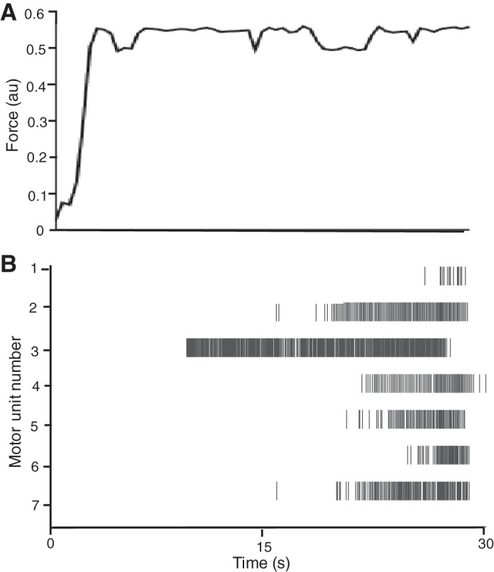
A: force exerted by a subject during a ramp-and-hold task to a target force of 10% MVC with the elbow flexors. B: Raster of discharge times for 7 motor units in the long head of biceps brachii. The motor unit activity was decomposed from high-density surface EMG recordings by a semiautomated blind source kernel compensation algorithm (Holobar and Zazula 2004; Negro et al. 2016b) during the hold phase of the task. The motor unit discharge times are shown from the last 20 s of the 30-s contraction.

Fig. 9.

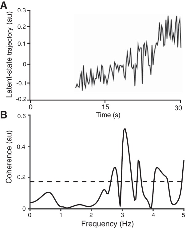
A: estimation of the single-dimension latent-state trajectory from the EM algorithm during the hold phase of the ramp-and-hold task (Buesing et al. 2012; Macke et al. 2011). The latent-state trajectory began after the participant had reached a relatively stable force due to the difficulty in discriminating motor unit discharge times (which are necessary to estimate the model parameters) during the ramp phase. B: coherence between force during the hold phase and the estimated latent-state trajectory, which reached a peak of 0.53 at ∼3 Hz.

DISCUSSION

The goal of this study was to demonstrate that a state-space model is able to estimate the synaptic input and its associated variance that is common to a pool of motor units. The study involved four different data sets, each chosen to evaluate the adequacy of the model to capture a physiologically relevant feature of a pool of motor neurons. First, a pool of motor units was modeled as a Poisson linear dynamic system excited by a one-dimensional common input. This data set created realistic motor unit discharge times and force characteristics observed during experimental studies. Second, the discharge characteristics of a pair of leaky integrate-and-fire neurons connected to an inhibitory interneuron was examined. This model captured the influence of the interposed Renshaw cell on the discharge rate of the receiving motor neuron and provided an intuitive understanding of how a state-space trajectory may activate such a pathway. Moreover, the state-space trajectory was not influenced by the duration of the simulation. Third, the spectral content of the CSTs for 10 integrate-and-fire neurons at two input current frequencies yielded similar high-frequency spectral content values for the lowest input current (0.1 nA). In contrast, the latent state-space model produced a state-space trajectory for the 10 neurons that differed for the two frequencies of input current at all amplitudes of input current. Finally, the common input observed in experimentally recorded discharge times of motor units in biceps brachii during a submaximal isometric contraction can be represented by a one-dimensional latent state.

State-space models have been used successfully to model unobserved neural activity that modulates neurons in cortical circuits (Cunningham and Yu 2014; Macke et al. 2015). These models combine a description of the coherent dynamics of an unobserved latent state, which is interpreted as the common input to the motor neuron pool in the current study, with the random nature of neural discharge activity (modeled as a Poisson process). The ability to quantify the common input distributed to motor neurons has been a matter of debate since the seminal work of Sears and Stagg (1976). Contemporary methods of quantifying neural drive have resulted in a renewed interest in the area (Farina and Negro 2012; Farina et al. 2017).

A key feature of current approaches to assess common input is the combination of the discharge times of many motor units into a cumulative spike train (Farina et al. 2014; Farina and Negro 2015) and examination of the coherence between fluctuations in the cumulative spike train and force during steady isometric contractions. This approach relies on approximating the motor unit pool as a linear filter excited by a common input and independent noise sources. As a result, the neural drive to the muscle comprises the common input signal and the common noise. This methodology has advanced the approach used to quantify the neural drive to muscle (Farina et al. 2014; Farina and Negro 2015), and the astounding ability to provide intuitive control of human-machine interfaces during reaching movements (Farina and Negro 2012; Farina et al. 2017).

Negro et al. (2016a) have proposed a method that quantifies the proportion of common input driving a pool of motor neurons, but this approach cannot distinguish between a common input signal and synaptic noise. Other contemporary techniques also rely on assumptions that are mathematically convenient but difficult to justify in terms of physiology, such as the linearity of the motor unit pool, the approximation of the neural discharges by continuous signals, and Gaussian distributions of noise sources. Although the cumulative spike train method (Farina and Negro 2014, 2015; Negro et al. 2016a) provides a reasonable estimate of the common input to motor neurons, a latent state-space model appears to be capable of detecting smaller differences in input current. Moreover, the frequency analysis used in the CST approach is sensitive to the duration of the signal, whereas the state-space approach is more versatile. As such, a state-space model provides a more sensitive method for approximating the common input and, separately, the synaptic noise (both shared and independent) received by a pool of motor neurons.

The EM algorithm provided reproducible estimates of the common input that activated the neurons in all simulations and during the experimental measurement of motor unit activity during a voluntary contraction. The time series of the latent state exhibited moderate coherence (0.53 at 3 Hz) with the applied force in the functional bandwidth of force production (De Luca and Erim 1994; Negro et al. 2016a), lending support to the concept that the fluctuations in the common input to motor neurons are directly observed in the force output (Castronovo et al. 2015; Farina et al. 2014; Farina and Negro 2015). The moderate coherence between the estimated latent state and the net force is remarkable because the discharge times from only seven motor units were observed during the experiment; it has been demonstrated that the ability to characterize the neural drive to muscle improves with an increase in the number of identified motor units (Farina et al. 2014; Farina and Negro 2015).

Although previous studies have demonstrated a link between force fluctuations during submaximal isometric contractions and oscillations in the neural drive to muscle (Castronovo et al. 2015; Negro et al. 2009), no study has differentiated between the control signal and the noise. In contrast, the covariance matrix, Q, in the state-space approach can be used to estimate the noise in the common input. The covariance could be used to examine the association between neural drive and force steadiness, even during long-lasting isometric contractions when the covariance in the input signal might change. This could be accomplished by separating the data (force and discharge times) into multiple segments in which the covariance is more stationary. Additionally, as suggested by Boonstra et al. (2016), the state-space model includes relevant physiological properties within the C matrix to encode the differential effects of the common input on motor units. The proposed model does not estimate specific physiological properties, but it does allow for entries in the C matrix to represent all key properties that influence the discharge of action potentials, such as input conductance and afterhyperpolarization duration (Gustafsson and Pinter 1984; Heckman and Enoka 2012; Henneman et al. 1965).

Although the state-space trajectory for the integrate-and-fire simulations contained frequency content that was greater than the injected current, its interpretation is intended to provide a qualitative approximation of the common input to the pool of motor neurons rather than quantify the frequency of the input. For example, the changes in the latent-state trajectory were more frequent for the 4-Hz current than the 3-Hz current (Fig. 7, C, F, and I). Moreover, the state-space trajectory for the experimental recordings of motor unit activity from a human subject did not include an input current with high spectral content. The higher frequency oscillations seen in the integrate-and-fire simulations could be due to overfitting of the parameters due to the relatively stable statistical structure of the simulated discharge times. These higher frequency oscillations were absent in the state-space trajectory for the experimental recording and the 120 simulated units.

The results from the simulations using relatively few parameters compared well with experimental data. For example, the variance in the estimated latent input signal decreased with an increase in target force for the 120 motor units simulated as a Poisson linear dynamic system, which has been demonstrated experimentally (Castronovo et al. 2015). Specifically, the coherence between cumulative spike trains of motor units increased with greater target forces (≤75%) and at the end of submaximal isometric contractions sustained until failure. These results suggest that the proportion of common input increases with net synaptic input. Additionally, the variability in force from the 120 motor units simulated as a Poisson linear dynamical system was within the experimentally reported range of values during steady isometric contractions for the first dorsal interosseus (Galganski et al. 1993; Moritz et al. 2005). The force variability of the simulated contractions, when expressed as the coefficient of variation for force, was greatest at low force outputs (5.9 ± 0.5% at 5% MVC) and decreased at greater target forces (2.1 ± 0.2% at 30% MVC).

Moreover, the present study demonstrated that the discharge times for a motor neuron receiving inhibitory input, such as is provided by Renshaw cells (Pratt and Jordan 1987), can be simulated with the state-space model. The parameters of the state-space model estimated from the discharge times of the pair of integrate-and-fire motor neurons with negative feedback were solved using the interconnectivity term within the model and produced a moderate peak in coherence (0.58) near the input frequency. Additionally, Fig. 6 demonstrates how latent-state trajectory fluctuates when the injected current (control signal + common noise) is greatest. These results indicate that a state-space model can identify the input to a system of neurons with a negative feedback pathway.

Similarly to the simulations, the estimated parameters from the motor unit activity during a voluntary contraction provided an intuitively accurate representation of the common input. The magnitude of the common input gradually increased over the course of the 20-s contraction. Experimental studies demonstrate the recruitment of additional motor units during the later stages of fatiguing contractions (Carpentier et al. 2001; Enoka et al. 1989; Person and Kudina 1972), which was seen in the present study (Fig. 8B, motor unit 1) and expressed in the model as an increase in the magnitude of the common input.

The present study proposes a method to analyze motor unit discharge times and quantify the trajectory and variance of the common input underlying the discharge activity of a pool of motor units. The physiologically plausible model represents the discharge times of motor neurons as a discrete process and does not require modeling neuron activity as a continuous time signal or approximating the motor neuron pool with a linear filter. The feasibility of an EM algorithm to estimate a latent input was demonstrated with two computational simulations and the discharge times of seven motor units during a ramp-and-hold voluntary contraction. Importantly, the coherence between the one-dimension latent input and the applied force showed a relatively high coherence in the critical bandwidth for force control. The present study demonstrates that a state-space model can be used to estimate an unobserved latent input signal that modulates the discharge times of the motor units even from relatively brief signals. Furthermore, the approach yields an independent estimate of the variance of the input, which may provide an index of the synaptic noise within the input signal. The approach could be used to quantify changes in the common input and the variability in the synaptic inputs across a range of conditions.

Conclusion.

A Poisson linear dynamic system can replicate the motor unit discharge times and muscle force characteristics observed experimentally during low-force steady contractions. The parameters of the model quantify a common input signal and the synaptic noise inherent in signal transmission to motor neurons. This approach can be used to quantify the common input received by pools of motor neurons on a trial-by-trial basis during brief and long-lasting voluntary isometric contractions.

DISCLOSURES

No conflicts of interest, financial or otherwise, are declared by the authors.

AUTHOR CONTRIBUTIONS

D.F.F., F.G.M., and R.M.E. conceived and designed research; D.F.F. and N.N. performed experiments; D.F.F. and N.N. analyzed data; D.F.F., F.G.M., and R.M.E. interpreted results of experiments; D.F.F. and R.M.E. prepared figures; D.F.F., F.G.M., and R.M.E. drafted manuscript; D.F.F., F.G.M., N.N., and R.M.E. edited and revised manuscript; D.F.F., F.G.M., N.N., and R.M.E. approved final version of manuscript.

REFERENCES

- Adrian ED, Bronk DW. The discharge of impulses in motor nerve fibres: Part II. The frequency of discharge in reflex and voluntary contractions. J Physiol 67: 119–151, 1929. [PMC free article] [PubMed] [Google Scholar]
- Ahmadian Y, Pillow JW, Paninski L. Efficient Markov chain Monte Carlo methods for decoding neural spike trains. Neural Comput 23: 46–96, 2011. doi: 10.1162/NECO_a_00059. [DOI] [PMC free article] [PubMed] [Google Scholar]
- Archer E, Koster U, Pillow J, Macke JH. Low-dimensional models of neural population activity in sensory cortical circuits. NIPS 27: 343–351, 2014. [Google Scholar]
- Barry BK, Pascoe MA, Jesunathadas M, Enoka RM. Rate coding is compressed but variability is unaltered for motor units in a hand muscle of old adults. J Neurophysiol 97: 3206–3218, 2007. doi: 10.1152/jn.01280.2006. [DOI] [PubMed] [Google Scholar]
- Berg RW, Ditlevsen S, Hounsgaard J. Intense synaptic activity enhances temporal resolution in spinal motoneurons. PLoS One 3: e3218, 2008. doi: 10.1371/journal.pone.0003218. [DOI] [PMC free article] [PubMed] [Google Scholar]
- Bigland B, Lippold OC. Motor unit activity in the voluntary contraction of human muscle. J Physiol 125: 322–335, 1954. [DOI] [PMC free article] [PubMed] [Google Scholar]
- Boonstra TW, Farmer SF, Breakspear M. Using computational neuroscience to define common input to spinal motor neurons. Front Hum Neurosci 10: 313, 2016. doi: 10.3389/fnhum.2016.00313. [DOI] [PMC free article] [PubMed] [Google Scholar]
- Bremner FD, Baker JR, Stephens JA. Variation in the degree of synchronization exhibited by motor units lying in different finger muscles in man. J Physiol 432: 381–399, 1991. doi: 10.1113/jphysiol.1991.sp018390. [DOI] [PMC free article] [PubMed] [Google Scholar]
- Buesing L, Macke JH, Sahani M. Spectral learning of linear dynamics from generalised-linear observations with application to neural population data. NIPS 25: 1691–1699, 2012. [Google Scholar]
- Carpentier A, Duchateau J, Hainaut K. Motor unit behaviour and contractile changes during fatigue in the human first dorsal interosseus. J Physiol 534: 903–912, 2001. doi: 10.1111/j.1469-7793.2001.00903.x. [DOI] [PMC free article] [PubMed] [Google Scholar]
- Castronovo AM, Negro F, Conforto S, Farina D. The proportion of common synaptic input to motor neurons increases with an increase in net excitatory input. J Appl Physiol (1985) 119: 1337–1346, 2015. doi: 10.1152/japplphysiol.00255.2015. [DOI] [PubMed] [Google Scholar]
- Cunningham JP, Yu BM. Dimensionality reduction for large-scale neural recordings. Nat Neurosci 17: 1500–1509, 2014. doi: 10.1038/nn.3776. [DOI] [PMC free article] [PubMed] [Google Scholar]
- De Luca CJ, Erim Z. Common drive of motor units in regulation of muscle force. Trends Neurosci 17: 299–305, 1994. doi: 10.1016/0166-2236(94)90064-7. [DOI] [PubMed] [Google Scholar]
- De Luca CJ, LeFever RS, McCue MP, Xenakis AP. Control scheme governing concurrently active human motor units during voluntary contractions. J Physiol 329: 129–142, 1982. doi: 10.1113/jphysiol.1982.sp014294. [DOI] [PMC free article] [PubMed] [Google Scholar]
- Dempster AP, Laird NM, Rubin DB. Maximum likelihood from incomplete data via the EM algorithm. J Royal Stat Soc 39: 1–38, 1977. [Google Scholar]
- Dideriksen JL, Farina D, Baekgaard M, Enoka RM. An integrative model of motor unit activity during sustained submaximal contractions. J Appl Physiol (1985) 108: 1550–1562, 2010. doi: 10.1152/japplphysiol.01017.2009. [DOI] [PubMed] [Google Scholar]
- Enoka RM, Robinson GA, Kossev AR. Task and fatigue effects on low-threshold motor units in human hand muscle. J Neurophysiol 62: 1344–1359, 1989. [DOI] [PubMed] [Google Scholar]
- Farina D, Negro F. Accessing the neural drive to muscle and translation to neurorehabilitation technologies. IEEE Rev Biomed Eng 5: 3–14, 2012. doi: 10.1109/RBME.2012.2183586. [DOI] [PubMed] [Google Scholar]
- Farina D, Negro F. Common synaptic input to motor neurons, motor unit synchronization, and force control. Exerc Sport Sci Rev 43: 23–33, 2015. doi: 10.1249/JES.0000000000000032. [DOI] [PubMed] [Google Scholar]
- Farina D, Negro F, Dideriksen JL. The effective neural drive to muscles is the common synaptic input to motor neurons. J Physiol 592: 3427–3441, 2014. doi: 10.1113/jphysiol.2014.273581. [DOI] [PMC free article] [PubMed] [Google Scholar]
- Farina D, Vujaklija I, Sartori M, Kapelner T, Negro F, Jiang N, Bergmeister K, Andalib A, Principe J, Aszmann OC. Man/machine interface based on the discharge timings of spinal motor neurons after targeted muscle reinnervation. Nat Biomed Eng 1: 1–12, 2017. doi: 10.1038/s41551-016-0025. [DOI] [Google Scholar]
- Farmer SF, Bremner FD, Halliday DM, Rosenberg JR, Stephens JA. The frequency content of common synaptic inputs to motoneurones studied during voluntary isometric contraction in man. J Physiol 470: 127–155, 1993. doi: 10.1113/jphysiol.1993.sp019851. [DOI] [PMC free article] [PubMed] [Google Scholar]
- Feinstein B, Lindegård B, Nyman E, Wohlfart G. Morphologic studies of motor units in normal human muscles. Acta Anat (Basel) 23: 127–142, 1955. doi: 10.1159/000140989. [DOI] [PubMed] [Google Scholar]
- Fuglevand AJ, Lester RA, Johns RK. Distinguishing intrinsic from extrinsic factors underlying firing rate saturation in human motor units. J Neurophysiol 113: 1310–1322, 2015. doi: 10.1152/jn.00777.2014. [DOI] [PMC free article] [PubMed] [Google Scholar]
- Fuglevand AJ, Winter DA, Patla AE. Models of recruitment and rate coding organization in motor-unit pools. J Neurophysiol 70: 2470–2488, 1993. [DOI] [PubMed] [Google Scholar]
- Galganski ME, Fuglevand AJ, Enoka RM. Reduced control of motor output in a human hand muscle of elderly subjects during submaximal contractions. J Neurophysiol 69: 2108–2115, 1993. [DOI] [PubMed] [Google Scholar]
- Gustafsson B, Pinter MJ. An investigation of threshold properties among cat spinal alpha-motoneurones. J Physiol 357: 453–483, 1984. doi: 10.1113/jphysiol.1984.sp015511. [DOI] [PMC free article] [PubMed] [Google Scholar]
- Heckman CJ, Enoka RM. Motor unit. Compr Physiol 2: 2629–2682, 2012. doi: 10.1002/cphy.c100087. [DOI] [PubMed] [Google Scholar]
- Henneman E, Somjen G, Carpenter DO. Functional significance of cell size in spinal motoneurons. J Neurophysiol 28: 560–580, 1965. [DOI] [PubMed] [Google Scholar]
- Ho BL, Kalman RE. Effective construction of linear state variable models from input/output functions. Regelungstechnik 14: 545–548, 1966. [Google Scholar]
- Holobar A, Zazula D. Correlation-based decomposition of surface electromyograms at low contraction forces. Med Biol Eng Comput 42: 487–495, 2004. [DOI] [PubMed] [Google Scholar]
- Katz B, Miledi R. Membrane noise produced by acetylcholine. Nature 226: 962–963, 1970. doi: 10.1038/226962a0. [DOI] [PubMed] [Google Scholar]
- Kernell D, Monster AW. Threshold current for repetitive impulse firing in motoneurones innervating muscle fibres of different fatigue sensitivity in the cat. Brain Res 229: 193–196, 1981. [DOI] [PubMed] [Google Scholar]
- Kirkwood PA, Sears TA, Westgaard RH. Recurrent inhibition of intercostal motoneurones in the cat. J Physiol 319: 111–130, 1981. doi: 10.1113/jphysiol.1981.sp013895. [DOI] [PMC free article] [PubMed] [Google Scholar]
- Kuhn A, Aertsen A, Rotter S. Higher-order statistics of input ensembles and the response of simple model neurons. Neural Comput 15: 67–101, 2003. doi: 10.1162/089976603321043702. [DOI] [PubMed] [Google Scholar]
- Macke JH, Buesing L, Cunningham JP, Byron MY, Shenoy KV, Sahani M. Empirical models of spiking in neural populations. NIPS 24: 1350–1358, 2011. [Google Scholar]
- Macke JH, Buesing L, Sahani M. Estimating State and Parameters in State Space Models of Spike Trains. Advanced State Space Methods for Neural and Clinical Data. Cambridge, UK: Cambridge University Press, 2015. [Google Scholar]
- Mangion AZ, Yuan K, Kadirkamanathan V, Niranjan M, Sanguinetti G. Online variational inference for state-space models with point-process observations. Neural Comput 23: 1967–1999, 2011. doi: 10.1162/NECO_a_00156. [DOI] [PubMed] [Google Scholar]
- Milner-Brown HS, Stein RB, Yemm R. The contractile properties of human motor units during voluntary isometric contractions. J Physiol 228: 285–306, 1973. doi: 10.1113/jphysiol.1973.sp010087. [DOI] [PMC free article] [PubMed] [Google Scholar]
- Monster AW, Chan H. Isometric force production by motor units of extensor digitorum communis muscle in man. J Neurophysiol 40: 1432–1443, 1977. [DOI] [PubMed] [Google Scholar]
- Moritz CT, Barry BK, Pascoe MA, Enoka RM. Discharge rate variability influences the variation in force fluctuations across the working range of a hand muscle. J Neurophysiol 93: 2449–2459, 2005. doi: 10.1152/jn.01122.2004. [DOI] [PubMed] [Google Scholar]
- Negro F, Holobar A, Farina D. Fluctuations in isometric muscle force can be described by one linear projection of low-frequency components of motor unit discharge rates. J Physiol 527: 5925–5938, 2009. doi: 10.1113/jphysiol.2009.178509. [DOI] [PMC free article] [PubMed] [Google Scholar]
- Negro F, Yavuz US, Farina D. The human motor neuron pools receive a dominant slow-varying common synaptic input. J Physiol 594: 5491–5505, 2016a. doi: 10.1113/JP271748. [DOI] [PMC free article] [PubMed] [Google Scholar]
- Negro F, Muceli S, Castronovo AM, Holobar A, Farina D. Multi-channel intramuscular and surface EMG decomposition by convolutive blind source separation. J Neural Eng 13: 026027, 2016b. doi: 10.1088/1741-2560/13/2/026027. [DOI] [PubMed] [Google Scholar]
- Nordstrom MA, Fuglevand AJ, Enoka RM. Estimating the strength of common input to human motoneurons from the cross-correlogram. J Physiol 453: 547–574, 1992. doi: 10.1113/jphysiol.1992.sp019244. [DOI] [PMC free article] [PubMed] [Google Scholar]
- Paninski L, Ahmadian Y, Ferreira DG, Koyama S, Rahnama Rad K, Vidne M, Vogelstein J, Wu W. A new look at state-space models for neural data. J Comput Neurosci 29: 107–126, 2010. doi: 10.1007/s10827-009-0179-x. [DOI] [PMC free article] [PubMed] [Google Scholar]
- Partridge LD. Modification of neural output signals by muscles: a frequency response study. J Appl Physiol 20: 150–156, 1965. [DOI] [PubMed] [Google Scholar]
- Perkel DH, Gerstein GL, Moore GP. Neuronal spike trains and stochastic point processes. I. The single spike train. Biophys J 7: 391–418, 1967. doi: 10.1016/S0006-3495(67)86596-2. [DOI] [PMC free article] [PubMed] [Google Scholar]
- Person RS. Rhythmic activity of a group of human motoneurones during voluntary contraction of a muscle. Electroencephalogr Clin Neurophysiol 36: 585–595, 1974. doi: 10.1016/0013-4694(74)90225-9. [DOI] [PubMed] [Google Scholar]
- Person RS, Kudina LP. Discharge frequency and discharge pattern of human motor units during voluntary contraction of muscle. Electroencephalogr Clin Neurophysiol 32: 471–483, 1972. doi: 10.1016/0013-4694(72)90058-2. [DOI] [PubMed] [Google Scholar]
- Pnevmatikakis EA, Soudry D, Gao Y, Machado TA, Merel J, Pfau D, Reardon T, Mu Y, Lacefield C, Yang W, Ahrens M, Bruno R, Jessell TM, Peterka DS, Yuste R, Paninski L. Simultaneous denoising, deconvolution, and demixing of calcium imaging data. Neuron 89: 285–299, 2016. doi: 10.1016/j.neuron.2015.11.037. [DOI] [PMC free article] [PubMed] [Google Scholar]
- Powers RK, Dai Y, Bell BM, Percival DB, Binder MD. Contributions of the input signal and prior activation history to the discharge behaviour of rat motoneurones. J Physiol 562: 707–724, 2005. doi: 10.1113/jphysiol.2004.069039. [DOI] [PMC free article] [PubMed] [Google Scholar]
- Powers RK, Heckman CJ. Synaptic control of the shape of the motoneuron pool input-output function. J Neurophysiol 117: 1171–1184, 2017. doi: 10.1152/jn.00850.2016. [DOI] [PMC free article] [PubMed] [Google Scholar]
- Pratt CA, Jordan LM. Ia inhibitory interneurons and Renshaw cells as contributors to the spinal mechanisms of fictive locomotion. J Neurophysiol 57: 56–71, 1987. [DOI] [PubMed] [Google Scholar]
- Sears TA, Stagg D. Short-term synchronization of intercostal motoneurone activity. J Physiol 263: 357–381, 1976. doi: 10.1113/jphysiol.1976.sp011635. [DOI] [PMC free article] [PubMed] [Google Scholar]
- Smith AC, Brown EN. Estimating a state-space model from point process observations. Neural Comput 15: 965–991, 2003. doi: 10.1162/089976603765202622. [DOI] [PubMed] [Google Scholar]
- Townsend BR, Paninski L, Lemon RN. Linear encoding of muscle activity in primary motor cortex and cerebellum. J Neurophysiol 96: 2578–2592, 2006. doi: 10.1152/jn.01086.2005. [DOI] [PubMed] [Google Scholar]
- Truccolo W. Stochastic models for multivariate neural point processes: collective dynamics and neural decoding. Analysis of Parallel Spike Trains. New York: Springer, 2010, p. 321–341. [Google Scholar]
- Watanabe RN, Magalhães FH, Elias LA, Chaud VM, Mello EM, Kohn AF. Influences of premotoneuronal command statistics on the scaling of motor output variability during isometric plantar flexion. J Neurophysiol 110: 2592–2606, 2013. doi: 10.1152/jn.00073.2013. [DOI] [PubMed] [Google Scholar]
- Williams ER, Baker SN. Circuits generating corticomuscular coherence investigated using a biophysically based computational model. I. Descending systems. J Neurophysiol 101: 31–41, 2009. doi: 10.1152/jn.90362.2008. [DOI] [PMC free article] [PubMed] [Google Scholar]
- Windhorst U. Do Renshaw cells tell spinal neurones how to interpret muscle spindle signals? Prog Brain Res 80: 283–294, 1989. doi: 10.1016/S0079-6123(08)62222-0. [DOI] [PubMed] [Google Scholar]