Figure 1. Canonical correlation analysis (CCA) and hierarchical clustering define four connectivity-based biotypes of depression.

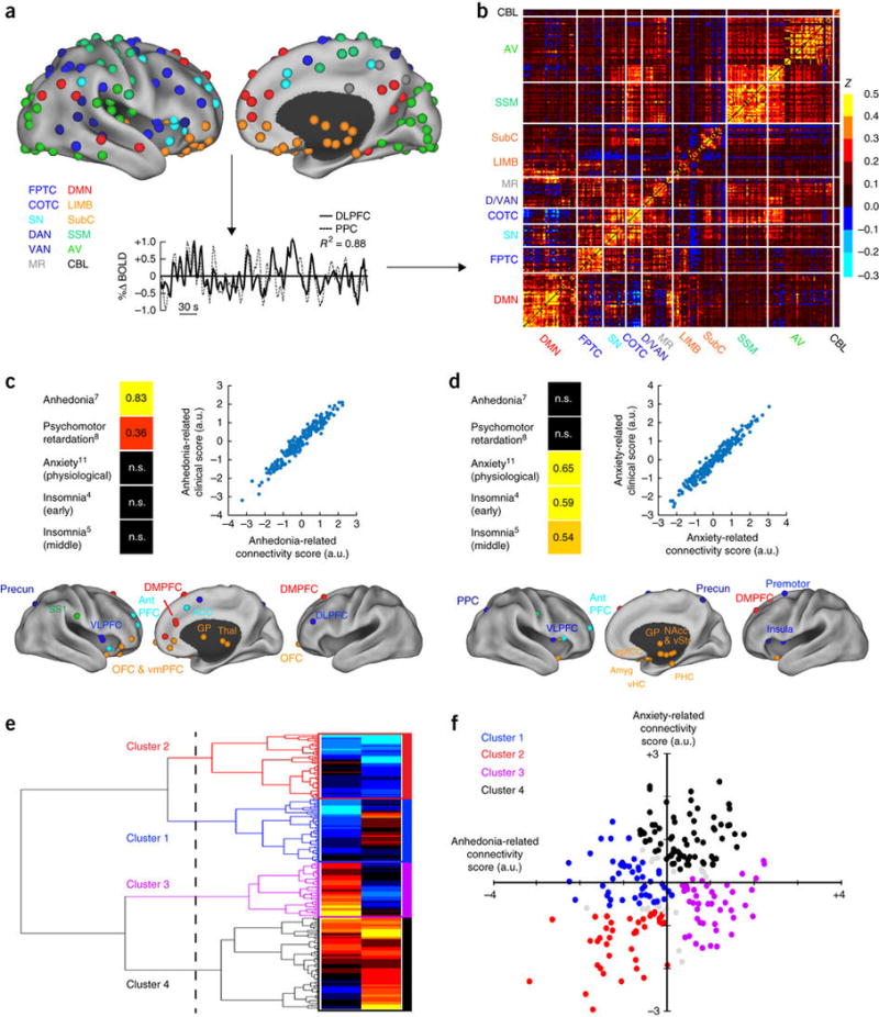
(a) Data analysis schematic and workflow. After preprocessing, BOLD signal time series were extracted from 258 spherical regions of interest (ROIs) distributed across the cortex and subcortical structures. The schematics (top) show lateral (left) and medial (right) views of right-hemisphere ROIs projected onto an inflated cortical surface and colored by functional network (lower left). Left-hemisphere ROIs (data not shown) were similar. For each subject, whole-brain functional-connectivity matrices were generated by calculating pairwise BOLD signal correlations between all ROIs, as in this example of correlated signals (r² = 0.88) for DLPFC (solid line) and PPC (dashed line) nodes of the FPTC network in a representative subject. (b) Whole-brain, 258 × 258 functional-connectivity matrix averaged across all healthy controls (n = 378 subjects). z = Fischer transformed correlation coefficient. (c,d) CCA was used to define a low-dimensional representation of depression-related connectivity features and identified an “anhedonia-related” component (canonical variate; c) and an “anxiety-related” component (d), represented by linear combinations of connectivity features that were correlated with linear combinations of symptoms. The scatterplots in c and d illustrate the correlation between low-dimensional connectivity scores and low-dimensional clinical scores for the anhedonia-related (r² = 0.91) and anxiety-related components (r² = 0.95), respectively (P < 0.00001, n = 220 patients with depression). To the left of each scatterplot, clinical score loadings (i.e., the Pearson correlation coefficients between specific symptoms and the anhedonia- or anxiety-related clinical score (canonical variate)) are depicted for those symptoms with the strongest loadings (HAMD item #, indicated by numbers in superscript; for all loadings on all symptoms, see Supplementary Fig. 2). Below each scatterplot, connectivity score loadings are summarized by depicting the neuroanatomical distribution of the 25 ROIs (top 10%) that were most highly correlated with each component (summed across all significantly correlated connectivity features for a given ROI), colored by network, as in a. Projections to the medial wall map are for both left- and right-hemisphere ROIs. (e) Hierarchical clustering analysis. The height of each linkage in the dendrogram represents the distance between the clusters joined by that link. For reference, the dashed line denotes 20 times the mean distance between pairs of subjects within a cluster. For analyses of additional cluster solutions and further discussion, see Supplementary Figure 3. (f) Scatterplot for four clusters of subjects along dimensions of anhedonia- and anxiety-related connectivity. Gray data points indicate subjects with ambiguous cluster identities (edge cases, cluster silhouette values < 0; n = 15, or 6.8% of all subjects). ACC, anterior cingulate cortex; amyg, amygdala; antPFC, anterior prefrontal cortex; a.u., arbitrary units; AV, auditory/visual networks; CBL, cerebellum; COTC, cingulo-opercular task-control network; D/VAN, dorsal/ventral attention network; DLPFC, dorsolateral prefrontal cortex; DMN, default-mode network; DMPFC, dorsomedial prefrontal cortex; FPTC, frontoparietal task-control network; GP, globus pallidus; LIMB, limbic; MR, memory retrieval network; NAcc, nucleus accumbens; OFC, orbitofrontal cortex; PPC, posterior parietal cortex; precun, precuneus; sgACC, subgenual anterior cingulate cortex; SS1, primary somatosensory cortex; SN, salience network; SSM, somatosensory/motor networks; subC, subcortical; thal, thalamus; vHC, ventral hippocampus; VLPFC, ventrolateral prefrontal cortex; VMPFC, ventromedial prefrontal cortex; vStr, ventral striatum; n.s., not significant. See Supplementary Table 4 for MNI coordinates for ROIs in b and c.