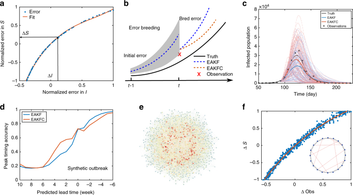
Fig. 1.

Error structure in SIRS model. a Error structure between the unobserved variable S and observed variable I following perturbations imposed 3 weeks prior to peak in a synthetic outbreak (N = 10⁵, S(0) = 0.5 N, I(0) = 1, L = 3.86 years, D = 2.27 days, R _0max = 3.79, R _0min = 0.97). The nonlinear error structure is estimated using a third-order polynomial, from which the error in S (∆S) can be inferred from the discrepancy of the observed variable with the synthetic observation (∆I). b Application of the breeding method to diagnose structural errors during the EAKF update. The initial random errors imposed at time t−1 evolve per model nonlinear dynamics until time t. c An example of EAKF and EAKFC prediction at 4 weeks prior to the peak for a simulated influenza outbreak. The dash lines depict the 300 ensemble predictions, while the solid lines are ensemble average trajectories. d Comparison of the fraction of EAKF and EAKFC peak timing predictions accurate within ±1 week of the synthetic peak. The results are averaged over 10³ SIRS-generated synthetic truths, each made with different parameters and initial conditions. For each synthetic outbreak, 100 independent predictions, each using a 300-member ensemble, are performed at each weekly observation time. e An example of an NW small-world network. f Error structure between the variable S and observation (weekly incidence) 3 weeks prior to peak in the small-world network model, fitted by a third-order polynomial. Inset is a schematic illustration of the NW small-world network. System state is the same as in a