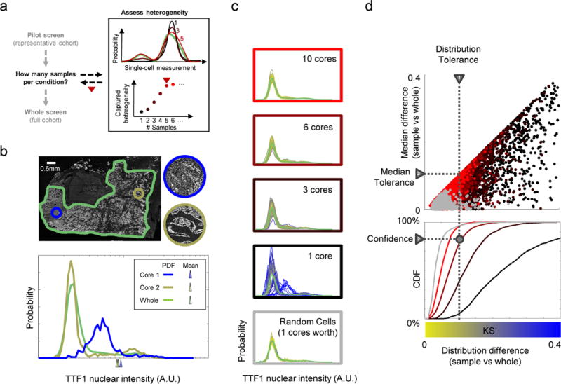
Figure 1. Sampling strategy to represent single-cell heterogeneity.

A) Overview of approach to determine how many samples (cores/replicates/draws) per condition are required for studies of heterogeneity. Top right: distributions of cellular phenotypes from different numbers of samples; bottom right: heterogeneity captured with different sample numbers. B) Samples that recover population averages may not capture heterogeneity. Papillary adenocarcinoma tumor (outlined in green) shows extensive heterogeneity in the staining of TTF1, but individual cores (circles) may not capture the full range of phenotypes. Bottom: distribution of TTF1 nuclear intensity (A.U.: arbitrary units, x-axis is on log scale) in the whole tissue and the cores. Cores and whole tissue have similar mean intensities (triangles below x-axis), yet differ greatly in their phenotypic distributions. C) Capturing whole-tissue heterogeneity depends on the number of cells sampled and the nature of the sampling. Plots: histograms of TTF1 distribution generated by repeated samplings of cells; colors based on agreement in distribution (blue or yellow show low or high (resp.) KS’ similarity) with whole tumor distribution (green curve). A single virtual core (~1000 cells on average) is unreliable, but spatially random draws with the same numbers of cells (bottom plot) captures heterogeneity as reliably as combining 10 virtual cores. D) Method for determining sample numbers needed to capture whole sample heterogeneity within a specified distribution tolerance (triangle “1”) at a desired level of confidence (triangle “2”). Upper scatter plot: comparison of whole tissue and samples generated as in B (point colors) based on their difference in distributions (x-axis: KS’ statistic) vs. medians (y-axis: deviation from the 50th percentile of the whole median). Differences in distributions places bounds on familiar quantities, such as differences in medians (triangle “1”; Methods). Bottom plot: confidence curves for achieving a desired KS’ tolerance as a function of sampling depth (number of cores) or type (core vs. random). This process allows rational user selection of the smallest number of samples (intersection of dotted lines) that capture whole specimen heterogeneity given desired tolerance and confidence levels. Given an existing library of specimens, confidence curves can be analyzed to estimate sampling depths of prospectively obtained samples for each choice of biomarker (e.g. Fig. 2C).