Figure 2.

Distributions of Spatial Footprint Similarities Modeled as a Weighted Sum of Two Subpopulations

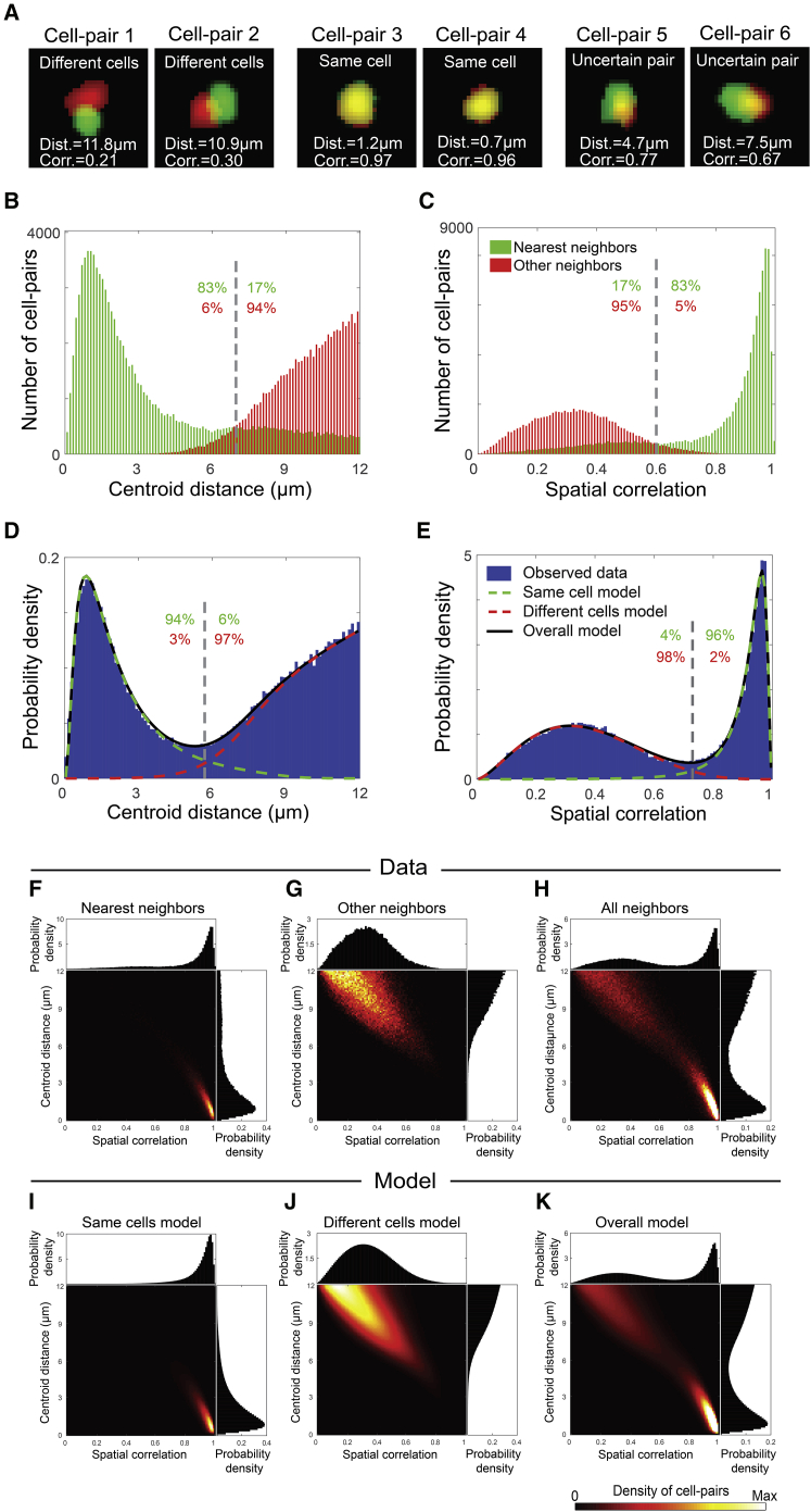
(A) Six examples of candidates to be the same cell, with their measured centroid distances (Dist.) and spatial correlations (Corr.). The spatial footprints are shown in red (session 1) and green (session 2).

(B and C) Distribution of centroid distances (B) and spatial correlations (C) between pairs of nearest neighbors (green) and other neighbors (red) across sessions. Gray dashed lines show the intersection between the two distributions. The fraction of nearest neighbors (green) or other neighbors (red) above and below these intersections are indicated.

(D and E) Distributions of centroid distances (D) and spatial correlations (E) between all neighboring cell-pairs (blue bars) and the modeled distributions of same cells (dashed green curves), different cells (dashed red curves), and their weighted sum (solid black curves). Gray dashed lines show the intersection between the two models. Estimated fractions of same cells (green) or different cells (red) above and below these intersections are indicated.

(F–H) Joint and marginal distributions of centroid distances and spatial correlations between pairs of nearest neighbors (F), other neighbors (G), and all neighbors (H) across sessions.

(I–K) Modeled joint and marginal distributions of centroid distances and spatial correlations for same cells (I), different cells (J), and their weighted sum (K). In (H) and (K), the color scale was set to reach 0.25 of the maximal value to enable visualization of both subpopulations. Data and models in all panels are for 16 sessions recorded on 8 different days in the hippocampal CA1 of a mouse while freely exploring the same environments.

See also Figures S3, S4, S5, and S6.