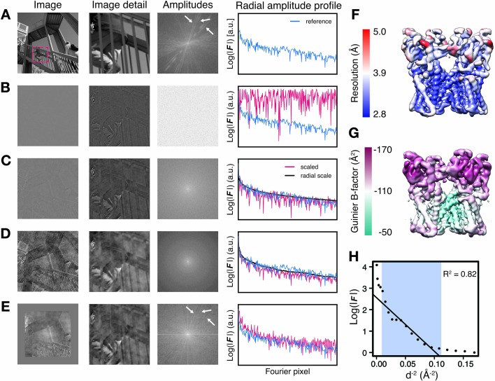
Figure 1. Illustration of local amplitude scaling (LocScale) using a 2D test image and determination local B-factors in cryo-EM maps.

(A) The original image (left), a magnified image detail (center left), the overall amplitude spectrum (center right) and the radially averaged amplitude profile (right) are displayed in panels along columns, respectively. Applied procedures are shown along rows. The radial amplitude profile of the reference, the scaled image and the applied scale are shown in blue, red and black, respectively. (B) Hybrid image resulting when amplitudes were replaced by random Gaussian noise and combined with phases from the original image in (A). The falloff of the amplitude profile of the hybrid image (red) is flat over the entire frequency range and hampers visual perception of image contrast. (C) Hybrid image from (B) when random amplitudes were scaled by a negative exponential estimated from the amplitude falloff of the original image. (D) Hybrid image from (C) with random amplitudes scaled by the average radial falloff profile from (A). (E) Hybrid image from (D) with amplitudes scaled locally to reference amplitudes from (A) computed in tiles of 128 × 128 pixel rolling windows. Note that diagonal lines in the amplitude spectrum (white arrows) arising from periodic image features are optimally recovered. Compare with the power spectrum of the original image. (F) Resolution estimates from local FSC calculation with a 24 Å sampling window mapped onto the surface representation of the TRPV1 channel (EMD-5778). (G) B-factors determined from local Guinier fitting in 24 Å sampling window mapped onto the surface representation of the TRPV1 channel (EMD-5778). (H) Guinier plot for a representative density window used for local B-factor estimation in (G). The linear falloff estimated from least squares fitting to the data is shown as straight line. The fitting interval ranging from 10 Å to the locally estimated resolution (here 3.1 Å) is highlighted in blue.

Figure 1—figure supplement 1. Local B-factor estimation by Guinier fitting.

(A) Coefficient of determination (R²) from local Guinier fitting mapped onto the molecular surface to TRPV1. (B) Distribution of B-factors estimated from local Guinier fitting mapped onto the molecular surfaces of γ-secretase, β-galactosidase and Pol III. (C) Coefficient of determination (R²) from local Guinier fitting as shown in (B) mapped onto the molecular surfaces of γ-secretase, β-galactosisdase and Pol III. (D) Local FSC curve shown for a representative 35 Å density window of Pol III. The estimated resolution is 6.6 Å based on FSC_0.143 threshold and 3σ criterion. (E) Guinier plot of the density window in (D). The linear falloff estimated from least squares fitting to the data is shown as straight line. The fitting interval ranging from 10 Å to the locally estimated resolution (here 6.6 Å) is highlighted in blue.