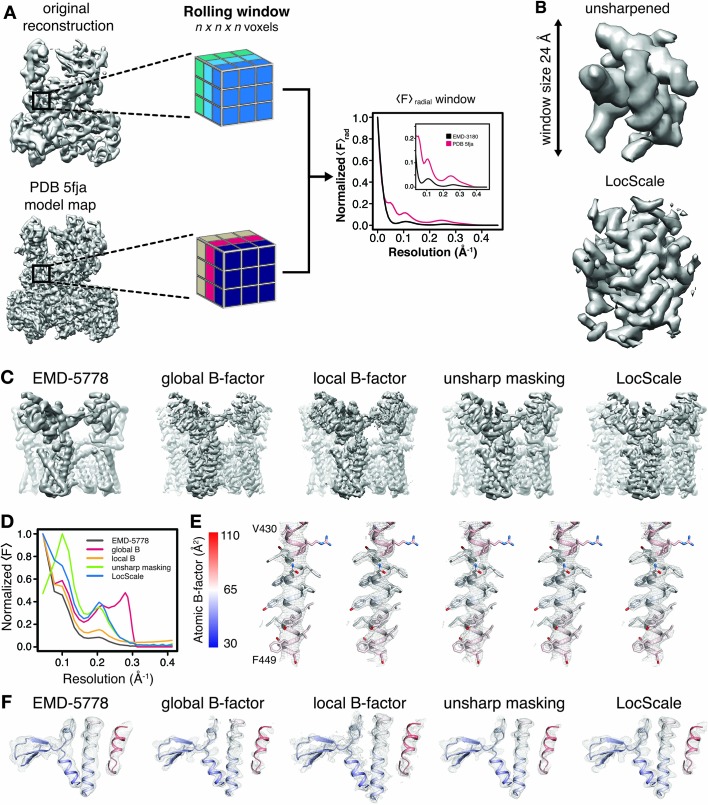
Figure 2. Generation of 3D LocScale density maps and comparison of global and local sharpening procedures.
(A) Schematic illustration of the LocScale procedure for a Pol III density map. Two equivalent map segments (rolling windows) are extracted from the original 3D reconstruction of EMD-3180 (top) and a map simulated from the atomic model (PDB ID 5fja) (bottom). For each rolling window, the radially averaged structure factor profile is computed and used to scale the amplitudes of the corresponding window of the original reconstruction. Note, the fine structure of the model amplitudes has a characteristic profile in the resolution range <10 Å due to protein secondary structure and deviates from a simple exponential falloff (inset). (B) Effect of amplitude scaling illustrated for an exemplary density window. The density contained within a window cube is shown before (unsharpened) and after (LocScale) application of amplitude scaling. The central voxel of the rolling window is assigned the map value after amplitude scaling. The procedure is repeated by moving the window along the map until each voxel has been assigned a density value based on the locally estimated contrast. (C) Side views of TRPV1 densities obtained with different sharpening methods. Far left, EMD-5778 unsharpened; left, global Guinier B-factor −100 Å2; middle, local Guinier B-factor; right, unsharp masking and far right, LocScale sharpening. (D) Radial amplitude profiles of the respective maps shown in (C). (E) Mesh representation of the densities for transmembrane residues 430–449 superposed on the atomic model (color-coded by atomic B-factor). The order from left to right is the same as in (C) and (F). Side chains are shown in stick representation. (F) Mesh representation for a peripheral density region superposed on the atomic model shown in ribbon representation and color-coded by atomic B-factor. B-factor scale as in (E).


