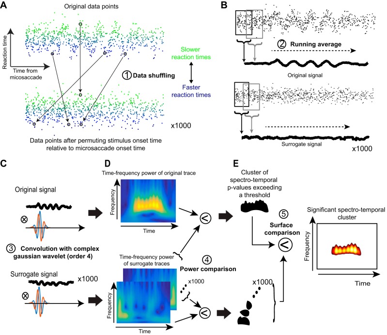
Fig. 2.

Steps used for time-frequency analyses in our study. A: we collected all trials and plotted each trial’s RT (as in the case of experiment 1) as a function of target onset time relative to a microsaccade. In this illustrative example, we show artificial data that have an underlying oscillatory pulse embedded in noise. Bottom: we shuffled the data in time, and we did this 1,000 times to obtain 1,000 surrogate data sets. B: we filtered the data using a running average to obtain a time course of fluctuations in the real data (top) and also for each of the 1,000 surrogate data sets. C: we then convolved each of the time course traces with a complex Gaussian wavelet of order 4. D: this allowed us to obtain time-frequency power spectra. For the real data, high power was observed during the interval in which an oscillation pulse was present in the original signal. The surrogate data sets had high power at random places in the time-frequency plots. E: we established statistical significance, with corrections for multiple comparisons, by finding a cluster in 2-dimensional time-frequency space in the original data set that was unlikely to be observed by chance from similar clusters observed in the surrogate data sets. We then plotted this “outlying” cluster with its associated P values as the significant cluster of spectrotemporal oscillation.