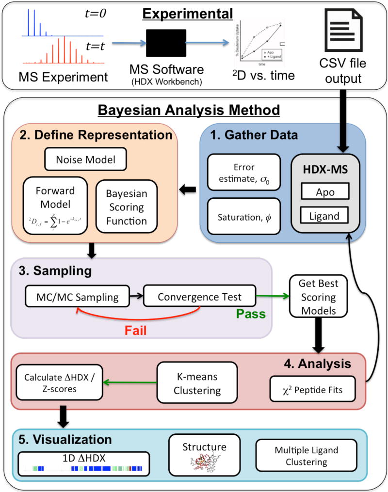
Figure 1. Method Flowchart.
Experimental: The method uses MS data that is analyzed by instrument-specific software, such as HDX Workbench, to produce 2D incorporation data vs. time. The resulting .csv files or modified .csv files are used as input into the Bayesian method. Bayesian Method: Step 1; Data (information) is gathered, including the HDX-MS 2D incorporation data for both apo and liganded (or perturbed) states as well an estimate for the error, σ0, and deuterium saturation level, ϕ, and the prior probabilities chosen for these two parameters (as described in the text). Step 2: The representation of the system is defined, beginning with the Forward Model, which, for this implementation is defined by the residue-resolved exchange rate chosen from a finite grid of values. The Noise model is defined as described in the text. This model defines the scoring function for each peptide. The Bayesian scoring function is then constructed by combining the scoring functions for all peptides, the noise model and prior probabilities. Step 3: A MC algorithm is used to sample the landscape of the Bayesian scoring function until a convergence criteria is passed. From this, a set of the best scoring models from each state are passed to Step 4. Analysis; where the individual experimental data points are compared to the top scoring models and clustering is performed to identify potential multi-state solutions. Analysis may show that more data need to be collected (if results are too imprecise) or that certain data points are inconsistent with the rest of the data. Finally, the ΔHDX and Z-scores are calculated between each state and visualized in Step 5 via a 1D plot, and on a 3D structure if available. Also, downstream analysis such as multiple ligand clustering can be performed.

