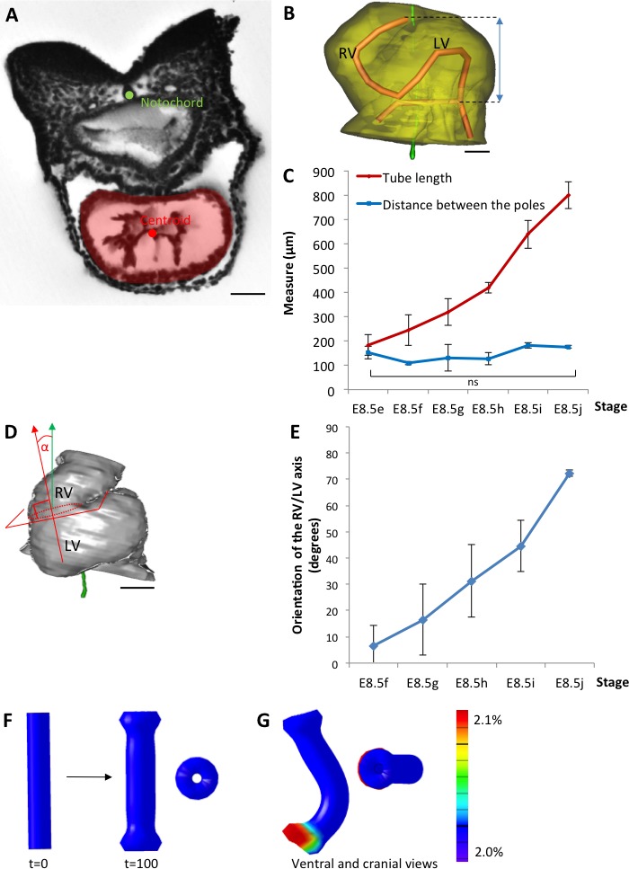
Figure 2. The heart tube elongates and loops between fixed poles.

(A) HREM image of an embryo section at E8.5f, with the notochord (green dot) and the centroid (red dot) of the myocardial tube (pale red) outlined. (B) Ventral view of a 3D reconstruction of the heart tube at E8.5i, aligned with the notochord vertical (green), showing the axis of the myocardial tube (red) used for the measurement of its length, and the distance between its poles (blue double-arrow). The measures were taken between the top of the arterial pole and the bifurcation between the two atrial regions at the venous pole. The distance between the poles was measured after projection onto the notochord. (C) Comparison between the tube length (red) and the distance between the poles (blue) during heart development. (D) Ventral view of a 3D reconstruction of the heart tube at E8.5h, aligned with the notochord vertical (green), showing the measurement of the orientation of the right ventricle (RV)-left ventricle (LV) axis. The perpendicular (red arrow) to the section of the interventricular sulcus (dotted circle) was drawn and its angle with the notochord (green arrow) was calculated. The measure was taken after projection onto the frontal plane. (E) Inclination of the right ventricle (RV)-left ventricle (LV) axis when looping progresses from a cranio-caudal (0°) towards a left-right orientation (90°). (F) Computer simulation of shape changes, in 3D, with a Finite Element model, seen from ventral (left) and cranial (right) views at step 100. Starting from a straight tube (t = 0), the simulation was run under the hypothesis of a tube growing homogenously between fixed poles, in the absence of any asymmetry. (G) Similar computer simulation, but with a small (5%) left-right asymmetry at one pole, mimicking stochastic, naturally occurring, left-right variations. The coloured scale of longitudinal growth used in the simulations is indicated on the right. Means and standard deviations are shown, with n = 3 for each point. Scale bar: 50 μm (A,B), 100 µm (D).
