. 2017 Dec 5;6:e22901. doi: 10.7554/eLife.22901

Figure 5. Co-ordinated errors between the output and hidden layers. .

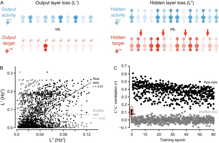
(A) Illustration of output loss function (L1) and local hidden loss function (L0). For a given test example shown to the network in a forward phase, the output layer loss is defined as the squared norm of the difference between target firing rates ϕ1 and the average firing rate during the forward phases of the output units. Hidden layer loss is defined similarly, except the target is ϕ0 (as defined in the text). (B) Plot of L1 vs. L0 for all of the ‘2’ images after one epoch of training. There is a strong correlation between hidden layer loss and output layer loss (real data, black), as opposed to when output and hidden loss values were randomly paired (shuffled data, gray). (C) Plot of correlation between hidden layer loss and output layer loss across training for each category of images (each dot represents one category). The correlation is significantly higher in the real data than the shuffled data throughout training. Note also that the correlation is much lower on the first epoch of training (red oval), suggesting that the conditions for credit assignment are still developing during the first epoch.

Figure 5—source data 1. Fig_5B.csv.
The first two columns of the data file contain the hidden layer loss (L0) and output layer loss (L1) of a one hidden layer network in response to all ‘2’ images in the MNIST test set after one epoch of training. The last two columns contain the same data, except that the data in the third column (Shuffled data L0) was generated by randomly shuffling the hidden layer activity vectors. Fig_5C.csv. The first 10 columns of the data file contain the mean Pearson correlation coefficient between the hidden layer loss (L0) and output layer loss (L1) of the one hidden layer network in response to each category of handwritten digits across training. Each row represents one epoch of training. The last 10 columns contain the mean Pearson correlation coefficients between the shuffled hidden layer loss and the output layer loss for each category, across training. Fig_5S1A.csv. This data file contains the maximum eigenvalue of (I-Jβ¯Jγ¯)T(I-Jβ¯Jγ¯) over 60,000 training examples for a one hidden layer network, where Jβ¯ and Jγ¯ are the mean feedforward and feedback Jacobian matrices for the last 100 training examples.
DOI: 10.7554/eLife.22901.009

Figure 5.

Figure 5—figure supplement 1. Weight alignment during first epoch of training.
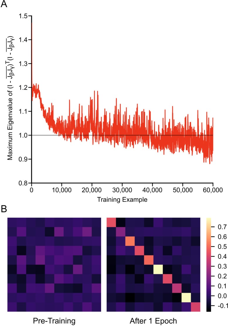
Figure 5—figure supplement 1.

(A) Plot of the maximum eigenvalue of (I-Jβ¯Jγ¯)T(I-Jβ¯Jγ¯) over 60,000 training examples for a one hidden layer network, where Jβ¯ and Jγ¯ are the mean feedforward and feedback Jacobian matrices for the last 100 training examples. The maximum eigenvalue of (I-Jβ¯Jγ¯)T(I-Jβ¯Jγ¯) drops below one as learning progresses, satisfying the main condition for the learning guarantee described in Theorem one to hold. (B) The product of the mean feedforward and feedback Jacobian matrices, Jβ¯Jγ¯, for a one hidden layer network, before training (left) and after 1 epoch of training (right). As training progresses, the network updates its weights in a way that causes this product to approach the identity matrix, meaning that the two matrices are roughly inverses of each other.