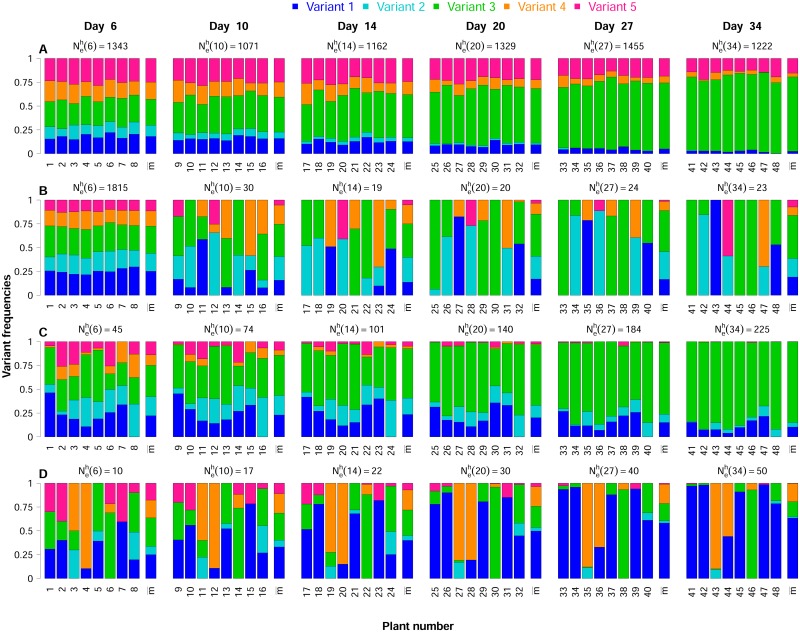
Fig 3. Contrasting datasets obtained in numerical experiment 1.

For each dataset (series A to D), the composition of eight populations was observed at six sampling dates, from 6 to 34 days post-inoculation, in independently sampled hosts. Within each plot, each bar represents the composition of the population in one plant at one date, and the last bar shows the mean frequencies over these populations. The color code at the top is used to distinguish the five variants. The harmonic mean of effective population size is indicated in the main title of each plot. The parameter values used for the simulations are: series (A) r = (0.971, 0.92, 1.09, 0.992, 1.027), $N_e^{IO}=1343$, $N_e^{S_1}=822$; series (B) r = (1.05, 1.005, 1.077, 0.963, 0.904), $N_e^{IO}=1815$, $N_e^{S_1}=12$; series (C) r = (1.045, 1.031, 1.12, 0.879, 0.924), $N_e^{IO}=45$, $N_e^{S_1}=1473$; series (D) r = (1.105, 0.943, 0.999, 1.041, 0.912), $N_e^{IO}=10$, $N_e^{S_1}=1025$. Note that $N_e^{S_1}$ is used for the iterative computation of a sequence of effective population sizes varying each five generations during the systemic infection stage.