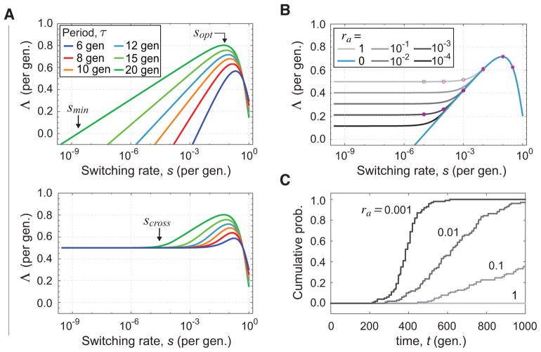
FIG. 2.

Fitness landscape for evolution of stochastic switching rates, for different stringency of selective bottlenecks. (A) Fitness landscape with a strong selective bottleneck (r_a = 0, upper panel) or a non-selective bottleneck (r_a = 1, lower panel). Each panel shows the long-term growth rate Λ as a function of switching rate s for different durations of proliferation τ, for transmission probability r_b = 1. We use f = 1 so that rates are expressed per generation. (B) Dependence of the fitness landscape for increasingly stringent bottleneck selection via decreasing r_a. Full (open) pink circles indicate the expected long-term growth rate using τ = 12 generations for strains with different switching rates with (without) bottleneck selection, showing that stronger selective bottlenecking leads to a steeper landscape and predicting faster evolution. (C) Evolutionary dynamics of stochastic switching rates for τ = 12 gen. Curves show the cumulative probability of fixation of the optimal switching strain (s = 0.1) over the set of simulations for the given value of r_a, each of which were initialized with a single cell of the lowest switching strain (s = 10⁻⁵). Mutations that alter switching rates occur with rate μ = 10⁻⁵ (reversibly), and change the switching rate by an order of magnitude. Six different switching rates can occur, at the values indicated by circles in panel B. The average population size in simulations is 10⁷ − 10⁸ cells. Fixation is defined as reaching a frequency greater than 0.9 in the population. Each curve is computed using at least 100 simulations. Each simulation was run for 1000 generations. For the values of r_a shown, extinction occurred in < 2% of simulation runs, and those runs were not used for analysis. The network of genotypes and phenotypes, average traces of simulated dynamics, and further simulation details are given in Fig. S2 and Appendix D.