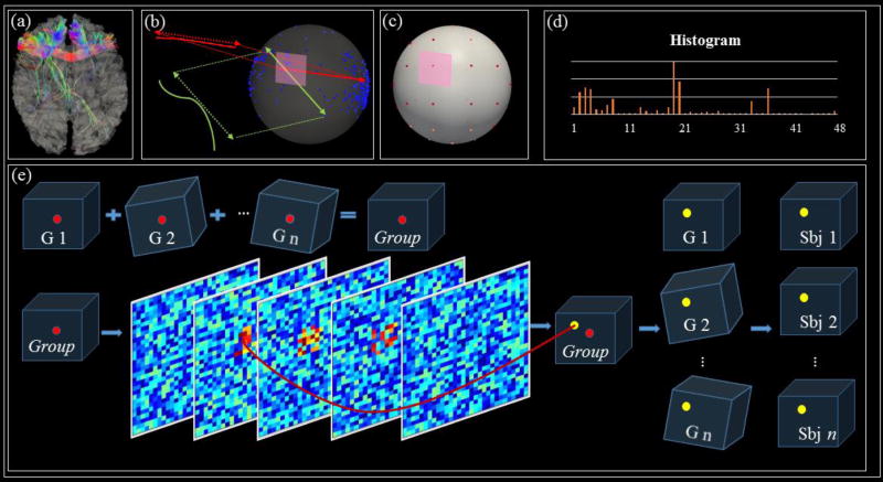
Fig 5.
The pipeline of ‘trace-map’ representation for representation of structural connectivity profile of landmarks. (a) An example of a landmark’s fiber bundle and cortical surface. (b) Points distribution by projection of the principal orientations of points of each fiber onto the unit sphere. (c) 48 equally-sized areas from one uniform sphere are shown. (d) 48-dimension vectors are used to represent one landmark’s fiber bundles. (e) The optimization step. The red bubbles are the initial landmarks, and yellow bubbles represent the locations after optimization.G1, G2 … Gn are landmarks in common space, and are landmarks transformed into individual spaces.

