
Figure 5. Blind compressed sensing (BCS) of gene modules.
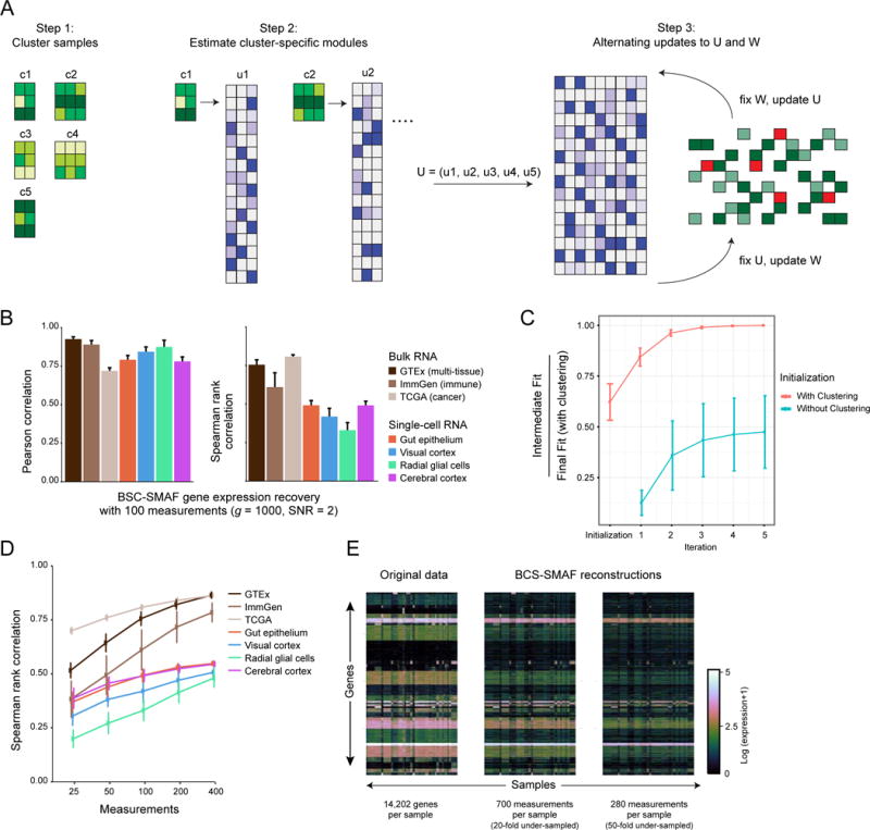
(A) BCS-SMAF steps. (1) Samples are clustered based on composite observations; (2) Small module dictionaries are estimated separately for each cluster, and concatenated into a large dictionary; (3) Procedure alternates over updates to the module dictionary and activity levels. (B–E) Performance of BCS-SMAF. (B) Bar plots of the Pearson (left) and Spearman (right) correlation coefficients (Y axis) between predicted and actual gene abundances. (C) Convergence of BCS-SMAF. The intermediate fit at each iteration as a fraction of the final fit (with clustering initialization) (Y axis), averaged across all datasets and random trials, when the algorithm can be initialized via clustering (red line), or randomly (teal line). (D) Spearman correlation coefficients (Y axis), as in (B), for varying numbers of composite measurements (X axis). Error bars in (B–D) represent one standard deviation across 50 random trials. (E) Original (left) expression levels for all 14,202 genes in GTEx and their corresponding predictions by applying BCS-SMAF to 700 (middle) and 280 (right) composite measurements.