. 2017 Nov 27;6:e28295. doi: 10.7554/eLife.28295

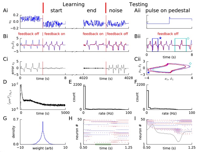
Figure 2. Learning non-linear dynamics via FOLLOW: the van der Pol oscillator.

(A-C) Control input, output, and error are plotted versus time: before the start of learning; in the first 4 s and last 4 s of learning; and during testing without error feedback (demarcated by the vertical red lines). Weight updating and error current feedback were both turned on after the vertical red line on the left at the start of learning, and turned off after the vertical red line in the middle at the end of learning. (A) Second component of the input u2. (B) Second component of the learned dynamical variable x^2 (red) decoded from the network, and the reference x2 (blue). After the feedback was turned on, the output tracked the reference. The output continued to track the reference approximately, even after the end of the learning phase, when feedback and learning were turned off. The output tracked the reference approximately, even with a very different input (Bii). With higher firing rates, the tracking without feedback improved (Figure 2—figure supplement 1). (C) Second component of the error ϵ2=x2-x^2 between the reference and the output. (Cii) Trajectory (x1(t),x2(t)) in the phase plane for reference (red,magenta) and prediction (blue,cyan) during two different intervals as indicated by and in Bii. (D) Mean squared error per dimension averaged over 4 s blocks, on a log scale, during learning with feedback on. Learning rate was increased by a factor of 20 after 1,000 s to speed up learning (as seen by the sharp drop in error at 1000 s). (E) Histogram of firing rates of neurons in the recurrent network averaged over 0.25 s (interval marked in green in H) when output was fairly constant (mean across neurons was 12.4 Hz). (F) As in E, but averaged over 16 s (mean across neurons was 12.9 Hz). (G) Histogram of weights after learning. A few strong weights |wij|>10 are out of bounds and not shown here. (H) Spike trains of 50 randomly-chosen neurons in the recurrent network (alternating colors for guidance of eye only). (I) Spike trains of H, reverse-sorted by first spike time after 0.5 s, with output component x^2 overlaid for timing comparison.

Figure 2.

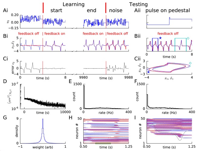
Figure 2—figure supplement 1. Learning van der Pol oscillator dynamics via FOLLOW with higher firing rates.

Figure 2—figure supplement 1.

Layout and legend of panels A-I are analogous to Figure 2A–I, except that maximum firing rates of neurons were larger (Figure 1—figure supplement 1) yielding approximately seven times the mean firing rates (for panels E and F, mean over 0.25 s and 16 s was 86.6 Hz and 87.6 Hz respectively), but approximately one-eighth the learning time, with constant learning rate.
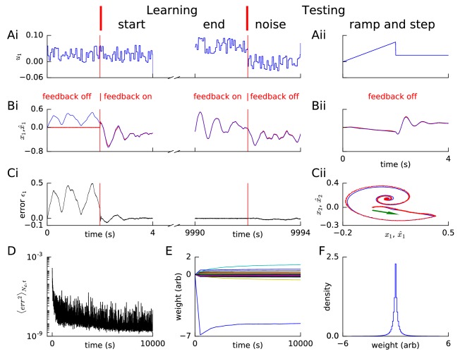
Figure 2—figure supplement 2. Learning linear dynamics via FOLLOW: 2D decaying oscillator.

Figure 2—figure supplement 2.

Layout and legend of panels (A-D) are analogous to Figure 2A–D, the green arrow in panel Cii shows the start of the trajectory of Bii. (E) A few randomly selected weights are shown evolving during learning. (F) Histogram of weights after learning. A few strong weights |wij|>6 are out of bounds and not shown here (cf. panel E).
Figure 2—figure supplement 3. Readout weights learn if recurrent weights are as is, but not if shuffled.
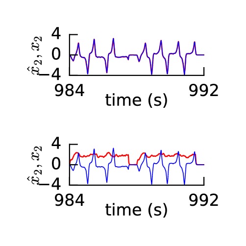
Figure 2—figure supplement 3.

(A-B) The readout weights were learned with a perceptron learning rule with the recurrent weights (A) as is after FOLLOW learning, or (B) shuffled after FOLLOW learning. A component of the output of the original FOLLOW-learned network (blue) and of the output of the network whose readout weights were trained (red) are plotted after the readout weights were trained for approximately 1,000 s. The readout weights learned if the recurrent weights were kept as is, but not if shuffled. Readout weights could also not be learned after shuffling only feedforward, shuffling both feedforward and recurrent connections.
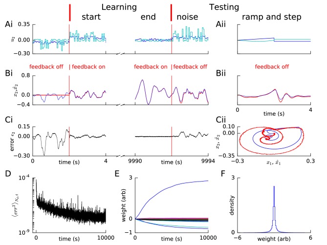
Figure 2—figure supplement 4. Learning non-linear feedforward transformation with linear recurrent dynamics via FOLLOW.

Figure 2—figure supplement 4.

Panels A-F are interpreted similar to Figure 2—figure supplement 2A–F, except in panel A, along with the input u2(t) (blue) to layer 1, the required non-linear transform g2(u(t))/20 is also plotted (cyan); and in panels E and F, the evolution and histogram of weights are those of the feedforward weights, that perform the non-linear transform on the input.
Figure 2—figure supplement 5. Feedforward weights are uncorrelated, while recurrent ones are correlated, when learning same recurrent dynamics but with different feedforward transforms.
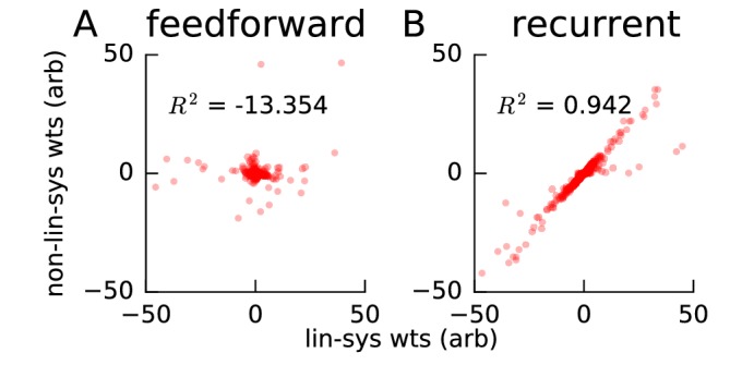
Figure 2—figure supplement 5.

The linear decaying oscillators system was learned for 10,000 s with either a non-linear or a linear feedforward transform. (A) The learned feedforward weights wilff were plotted for the system with the non-linear feedforward transform, versus the corresponding feedforward weights for the system with the linear feedforward transform. The feedforward weights for the two systems do not fit the identity line (coefficient of determination R2 is negative; R2 is not the square of a number and can be negative) showing that the learned feedforward transform is different in the two systems as expected. (B) Same as A, but for the recurrent weights in the two systems. The weights fit the identity line with an R2 close to one showing that the learned recurrent transform is similar in the two systems as expected. Some weights fall outside the plot limits.