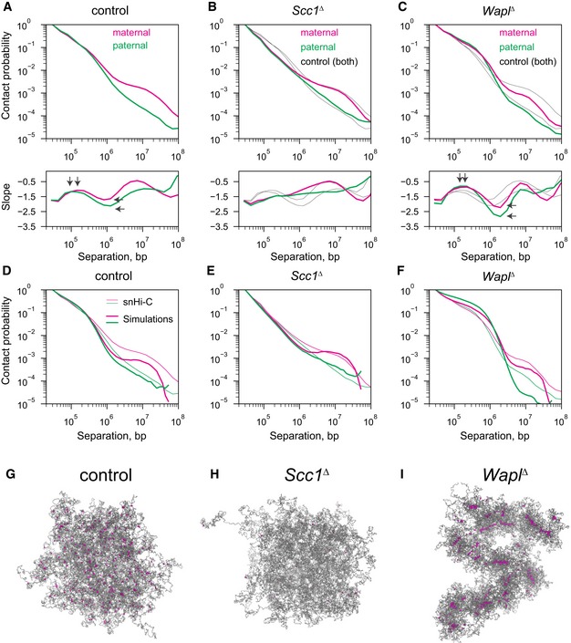
Figure 4. Differences in genome‐wide contact probability, P_c(s), for chromatin loci separated by genomic distances, s, between conditions.

• A–C
  Experimental P_c(s) for maternal and paternal chromatin for Scc1 control, Scc1 ^∆, and Wapl ^∆ conditions. Black solid lines in (B and C) show the control curves as a reference to guide the eye. Slopes of the log(P_c(s)) curves for each condition are shown in the subpanel below each P_c(s) plot. Vertical arrows on the slope subpanels indicate the maximum slope, which is used to infer the average size of cohesin‐extruded loops; this analysis indicates that the average extruded loop size is approximately 60–70 kb in control zygotes and increases in the Wapl ^∆ condition to over 120 kb. Horizontal arrows on the slope panels indicate the minimum slope, which can indicate cohesin linear density on the chromatin; notably, neither maternal nor paternal Scc1 ^∆ zygotes have a minimum slope suggesting very low cohesin density, whereas minima exist in both control and Wapl ^∆ conditions. Data are based on n(Wapl ^fl, maternal) = 7, n(Wapl ^fl, paternal) = 6, n(Wapl ^∆ , maternal) = 8, n(Wapl ^∆ , paternal) = 7, n(Scc1^fl, maternal) = 13, n(Scc1 ^fl, paternal) = 17, n(Scc1 ^∆, maternal) = 28, and n(Scc1 ^∆, paternal) = 17 nuclei, from at least two independent experiments using two to three females per genotype each.
• D–F
  Simulated chromatin P_c(s) for the control, Scc1 ^∆, and Wapl ^∆ conditions. Simulation P_c(s) curves shown in thick lines and experimental P_c(s) curves in thin lines.
• G–I
  Representative images of the simulated paternal chromatin fiber used for the P_c(s) calculations in panels (D–F). The chromatin fiber is colored in gray, and the locations of the cohesins are colored in purple.

Source data are available online for this figure.