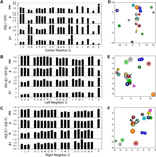
Figure 2.

Effects on the backbone conformational distribution from (A,D) the residue itself, (B,E) preceding, and (C,F) following residue. Populations of four regions with characteristic backbone torsion angles are evaluated: PPII, β, α_R, and type I β‐turn (β‐I) [marked in Fig. 1(A)]. (A) For each residue type X_i in the coil library, its impact on the backbone ϕ/ψ conformational distribution is evaluated by using the ratio of the normalized residue density (black bars) between subsets $\left\{X_i\right\}$ and all data {X} in the coil library. (B‐C) For each residue type Z, the ratio of the normalized residue density d, d(ϕ,ψ)/Σd(ϕ,ψ), between subsets $\{Z-\underset{¯}{X}\}$ (or $\{\underset{¯}{X}-Z\}$) and all data in the coil library $\{X-X\}$ are firstly calculated for its neighbor residue $\underset{¯}{X}$. The weighted averaged ratio < $d\{Z-\underset{¯}{X}\}$/ $d\{X-\underset{¯}{X}\}$> and < $d\{\underset{¯}{X}-Z\}$/ $d\{\underset{¯}{X}-X\}$> is then calculated and plotted (black bars) for each of the four ϕ/ψ regions, visualizing the impact of the preceding (B) and following residue (C) on the ϕ/ψ region populated by the center residue. The calculation is performed for five randomly selected two‐half subset of the random coil library, the average pairwise RMS deviation observed among these 10 sets of calculated density ratios is calculated and plotted (as error bars). Xaa‐Pro, Gly and Pro are excluded from the center residue set X. (D‐F) Multi‐dimensional scaling plots of average Hellinger distances between (D) any two center residues, (E) any pair of preceding, or (F) any pair of following residues. Hellinger distance maps (upscaled by a factor of 100) were derived as described by Ting et al.19 The radius of each bubble in the 2D map corresponds to half the positional uncertainty, as derived from jackknife analysis. Locations of Pro (at x,y = −34, 5) falls outside the box shown in (F), and Gly (at x,y = −52, 6) and Pro (at x,y = −2, −45) fall outside the box shown in (D). Clustering of the 20 residue types in the Hellinger maps is used to aid grouping of residues in (A‐C). Full sets of pairwise Hellinger distances are given in Supporting Information Table S7