Shape Matching and Registration by Data-driven EM

Abstract

In this paper, we present an efficient and robust algorithm for shape matching, registration, and detection. The task is to geometrically transform a source shape to fit a target shape. The measure of similarity is defined in terms of the amount of transformation required. The shapes are represented by sparse-point or continuous-contour representations depending on the form of the data. We formulate the problem as probabilistic inference using a generative model and the EM algorithm. But this algorithm has problems with initialization and computing the E-step. To address these problems, we define a discriminative model which makes use of shape features. This gives a hybrid algorithm which combines the generative and discriminative models. The resulting algorithm is very fast, due to the effectiveness of shape-features for solving correspondence requiring typically only four iterations. The convergence time of the algorithm is under a second. We demonstrate the effectiveness of the algorithm by testing it on standard datasets, such as MPEG7, for shape matching and by applying it to a range of matching, registration, and foreground/background segmentation problems.

1 Introduction

Shape matching is a very important problem in computer vision. The work in this paper treats shape matching as finding the best geometrical transformation between two shapes in the spirit of Grenander’s pattern theory [12].

There is a big literature on the different varieties of shape representations, matching criteria, and algorithms that have been applied to this problem. This includes representations such as Fourier analysis [43], moments [14], scale space [24], and level sets [27]. Some representations, such as FORMS [44] or shock-edit [33], explicitly represent the shape in terms of parts. Other approaches using chamfer matching [35] formulate the problem to enable rapid search through different appearances of the shape. Alternative approaches include manifold learning and metric embedding [15] and hierarchical structures with associative graphs [28]. For more details of shape representations and matching algorithms see recent survey papers [19,39]. Our approach is mostly closely related to the probabilistic formulation using free energies developed by [8,30,21] and the work on shape context [4].

We formulate the problem in terms of probabilistic inference using a generative model. This formulation involves hidden variables which indicate the correspondence between points on the two shapes. This leads naturally to an EM algorithm based on the free energy formulation [26]. Unfortunately computational issues make performing the E-step impractical and also give problems for initialization. We solve these problems by introducing a discriminative model which uses shape features. These shape features are less ambiguous for matching than points, and hence we call them informative features. This leads to a hybrid algorithm which combines the generative and discriminative models. See Tu et al [36] for more discussion of the trade-off between generative and discriminative methods.

Our approach helps unify existing work by Chui and Rangarajan [8] and Belongie et al [4]. We use a probabilistic formulation similar to Chui and Rangarajan but combine this with the shape features described by Belongie et al. This leads to an algorithm that has fewer iterations and better initialization than Chui and Rangarajan, while being better at dealing with uncertainty than Belongie et al.

Our approach represents the shapes in terms of points, which are supplemented by shape feature for the discriminative models. We use two types of representations – sparse-point and continuous-contour. The continuous-contour representation leads to better shape features, since the arc-length is known, but this representation is not always practical to compute. These representations are adequate for this paper, but their lack of ability to represent shape parts makes them unsuitable for matching shapes when parts can be missing (unlike methods such as [44,33]).

The structure of this paper is as follows. Section (2) gives the generative formulation of the problem. In section (3), we motivate the discriminative approach. Section (4) describes how the algorithm combines the two methods. In section (5) we give examples on a range of datasets and problems.

2 The Generative Formulation

The task of shape matching is to match two shapes, X and Y, and to measure the similarity between them. We refer to X as the target shape and Y as the source shape. We define the similarity measure in terms of the transformation that takes the source shape into the target, see figure 6. In this paper we use two types of transformation: (i) a global affine transformation A and (ii) a smooth non-rigid transformation f.

Fig. 6.

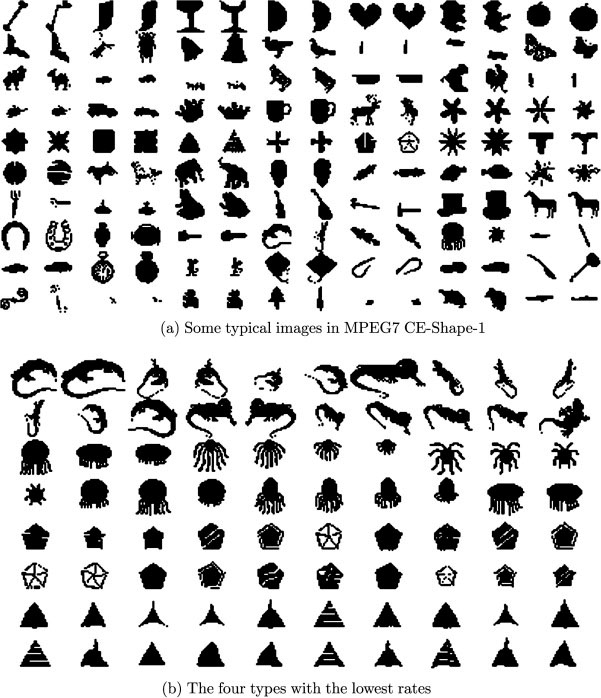
The MPEG7 CE-Shape-1.

2.1 Shape Representation

We use two types of shape representation in this paper: (I) sparse-point, and (II) continuous-contour. The choice will depend on the form of the data. Shape matching will be easier if we have a continuous-contour representation because we are able to exploit knowledge of the arc-length to obtain shape features which are less ambiguous for matching, and hence more informative, see section (3.1). But it may only be possible to compute a sparse-point representation for the target shape (e.g. the target shape may be embedded in an image and an edge detector will usually not output all the points on its boundary).

1. For the sparse-point representation, we denote the target and source shape respectively by:

   $$X=\{{\mathbf{x}}_i:i=1,\dots ,M\},\hspace{0.17em}\hspace{0.17em}\hspace{0.17em}\text{and\hspace{0.17em}}\hspace{0.17em}\hspace{0.17em}Y=\{{\mathbf{y}}_a:a=1,\dots ,N\}.$$ (1)

2. For the continuous-contour representation, we denote the target and source shape respectively by:

   $$X=\{\mathbf{x}(s):s\in [0,1]\},\hspace{0.17em}\hspace{0.17em}\hspace{0.17em}\text{and\hspace{0.17em}}\hspace{0.17em}\hspace{0.17em}Y=\{\mathbf{y}(t):t\in [0,1]\},$$ (2)

   where s and t are the normalized arc-length. In this case, each shape is represented by a 2D continuous-contour. By sampling points along the contour we can obtain a sparse-point representation X = {x_i : i = 1, …, M}, and Y = {y_a : a = 1, …, N}. But we can exploit the continuous-contour representation to compute additional features that depend on differentiable properties of the contour such as tangent angles.

2.2 The Generative Model

Our generative model for shape matching defines a probability distribution for generating the target X from the source Y by means of a geometric transformation (A, f). There will be priors P(A), P(f) on the transformation which will be specified in section (2.3).

We also define binary-valued correspondence variables {V_ai} such that V_ai = 1 if point a on the source Y matches point i on the target X. These are treated as hidden variables. There is a prior P(V) which specifies correspondence constraints on the matching (e.g. to constrain that all points on the source Y must be matched).

The choice of the correspondence constraints, as specified in P(V) is very important. They must satisfy a trade-off between the modeling and computational requirements. Constraints that are ideal for modeling purposes can be computationally intractable. The prior P(V) will be given in section (2.5) and the trade-off discussed.

The full generative model is P(X, V, A, f|Y) = P(X|Y, V, A, f)P(A)P(f)P(V), where the priors are given in sections (2.3), (2.5). The distribution P(X|Y, V, A, f) is given by:

$$\begin{array}{l}P(X|Y,V,\mathbf{A},\mathbf{f})=\frac{1}{Z}exp\{-E_G(X,Y,V,\mathbf{A},\mathbf{f})\},\hspace{0.17em}\hspace{0.17em}\hspace{0.17em}\text{where},\\ E_G(X,Y,V,\mathbf{A},\mathbf{f})=\sum _{i=1}^M\sum _{a=1}^N{V}_{ai}\left|\right|{\mathbf{x}}_i-\mathbf{A}{\mathbf{y}}_a-\mathbf{f}({\mathbf{y}}_a)|{|}^2.\end{array}$$ (3)

By using the priors P(A), P(f), P(V) and summing out the V’s, we obtain (this equation defines E_T [A, f; X, Y]):

$$P(X,\mathbf{A},\mathbf{f}|Y)=\sum _{V}P(X|Y,V,\mathbf{A},\mathbf{f})P(V)P(\mathbf{A})P(f)\triangleq \frac{1}{\widehat{Z}}exp\{-E_T[\mathbf{A},\mathbf{f};X,Y]\}$$ (4)

We define the optimal geometric transformation to be:

$$({\mathbf{A}}^{\ast },{\mathbf{f}}^{\ast })=arg\underset{\mathbf{A},\mathbf{f}}{max}P(X,\mathbf{A},\mathbf{f}|Y)=arg\underset{\mathbf{A},\mathbf{f}}{min}{E}_T[\mathbf{A},\mathbf{f};X,Y].$$ (5)

We define the similarity measure between shapes to be

$$S(X:Y)=E_T[{\mathbf{A}}^{\ast },{\mathbf{f}}^{\ast };X,T]=-logP(X,{\mathbf{A}}^{\ast },{\mathbf{f}}^{\ast }|Y)-log\widehat{Z}.$$ (6)

This is the negative logarithm of probability of generating the target X from the source Y by the optimal transformation, with the normalization constant Ẑ removed. This similarity measure will also correspond to the minimum of the free energy, see equation (12) (again with the normalization constant removed).

2.3 The Geometric Prior

The geometric transformation consists of a global (affine) transformation A and a smooth non-rigid transformation f (which includes a translation term). The prior on the non-rigid transformation f will enforce it to be smooth, and will be given at the end of this section. The prior on the affine transformation A is defined based on its decomposition into rotation angle θ, scaling S_x, S_y, and shear k. It encourages equal scaling both directions and favors limited shear.

More precisely, we decompose the affine transformation as follows:

$$\mathbf{A}=\left(\begin{array}{cc}{S}_x& 0\\ 0& S_y\end{array}\right)\left(\begin{array}{cc}cos\theta & -sin\theta \\ sin\theta & cos\theta \end{array}\right)\left(\begin{array}{cc}1& k\\ 0& 1\end{array}\right).$$ (7)

The prior on A is given by

$$p(\mathbf{A})\propto exp\{-E_A(\mathbf{A})\},\mathrm{\hspace{0.17em} }\text{and\hspace{0.28em}}{E}_A(\mathbf{A})=E_{\mathit{scale}}(S_x,S_y)+E_{\mathit{shear}}(k)+E_{\mathit{rot}}(\theta ),$$ (8)

where $E_{\mathit{scale}}(S_x,S_y)=b_1{(\frac{S_x-S_y}{S_x+S_y})}^2$, E_shear(s) = b₂k², and E_rot(θ) is constant (i.e. the prior on θ is the uniform distribution). In our experiments, we set b₁ = 1.0 and b₂ = 10.0.

The prior on the non-rigid transformation f is of form:

$$p(\mathbf{f})\propto exp\{-E_f(\mathbf{f})\}.$$ (9)

In this paper, we use the thin-plate-spline (TPS) kernel [5] where we impose that f is of form:

$$\mathbf{f}(x,y)=\sum _a{\mathbf{w}}^{a}U(x_a-x,y_a-y)+\mathbf{t},$$ (10)

where ${\mathbf{w}}^a=(w_x^a,w_y^a)$ are vector valued weights, x, y are the components of the vector y, U(x, y) = (x² + y²) log(x² + y²), t is translation, Σ_a w^a = 0, and ${\sum }_a{w}_x^a{x}_a={\sum }_a{w}_y^a{y}_a=0$. Then we define E_f by:

$$\begin{array}{l}{E}_f(\mathbf{f})=\lambda \iint {\left(\frac{{\partial }^2\mathbf{f}}{\partial x^2}\right)}^2+2{\left(\frac{{\partial }^2\mathbf{f}}{\partial x\partial y}\right)}^2+{\left(\frac{{\partial }^2\mathbf{f}}{\partial y^2}\right)}^2\mathit{dxdy}.\\ =\lambda \sum _{a,b=1}^N{\mathbf{w}}_a^{T}U({\mathbf{y}}_a-{\mathbf{y}}_b){\mathbf{w}}_b.\end{array}$$ (11)

We also considered an alternative energy function which encourages f to be small and smooth (Yuille and Grzywacz [41]). The small-and-smooth energy function usually gave similar results to the thin-plate-spline, but it required us to model the translation t separately. We will not discuss it further in this paper. Note that in our ECCV paper [37] our reported results were obtained using the TPS, but we erroneously stated that they were obtained using small-and-smooth.

2.4 The EM algorithm

We use the EM algorithm to estimate (A*, f*) = arg max_A,f P(X, A, f|Y), where the correspondence variables V are treated as hidden variables which are summed out.

It can be shown [26] that estimating (A*, f*) from P(X, A, f|Y) is equivalent to minimizing the EM free energy function:

$$\begin{array}{l}F(Q,\mathbf{A},\mathbf{f})=-logP(X,\mathbf{A},\mathbf{f}|Y)+\sum _{V}Q(V)log\frac{Q(V)}{P(V|X,Y,\mathbf{A},\mathbf{f})}\\ =-\sum _{V}Q(V)log\{P(X|Y,V,\mathbf{A},\mathbf{f})P(\mathbf{A})P(\mathbf{f})P(V)\}+\sum _{V}Q(V)logQ(V),\end{array}$$ (12)

where Q(V) is a distribution over the correspondence variables. The minimum of the free energy F(Q, A, f) is equal to min_A,f {− log P(X, A, f|Y)}.

The EM algorithm consists of two steps: (I) The M-step minimizes F(Q, A, f) with respect to (A, f) with Q(V) fixed and will be given in detail in section (4).(II) The E-step minimizes F(Q, A, f) with respect to Q(V) keeping (A, f) fixed. The E-step at iteration t can be expressed analytically as:

$$Q^t(V)=P(V|X,Y,{\mathbf{A}}^{t-1},{\mathbf{f}}^{t-1})$$ (13)

Unfortunately there are two difficulties with using the EM algorithm in the current form. Firstly, it requires good initialization or it will get stuck in a local maximum of P(X, A, f|Y). Secondly, the E-step is very difficult to compute unless we put restrictions on the prior P(V) which are so strong that they may degrade the quality of the result, see section (2.5). These problems motivate us to introduce a discriminative model, see section (3).

2.5 The Correspondence Constraints and P(V)

The prior P(V) enforces constraints on the correspondences between points on the target and the source. This leads to a trade-off between modeling and computational requirements.

From the modeling perspective, we would prefer constraints which are two-sided between the target and source. These constraints would enforce that most target and source points are matched, and would be flexible enough to allow for missing points. But imposing two-sided constraints makes the E-step of the EM algorithm impractical, because it is impossible to compute the right-hand side of equation (13).

One strategy to deal with this problem is by using a mean field theory approximation together with two-sided constraints. This strategy was used by Chui and Rangarajan [8] and was very successful. We will describe it at the end of this section.

Another strategy is to impose one-sided constraints which ensure that all points on the sources are either matched to points on the target, or are unmatched (and pay a penalty). In theory, this would allow situations where a single point of the target is matched to many points on the source, while many other target points are unmatched. In practice, the nature of the geometric transformations can prevent these situations from happening (since they correspond to highly improbable, or impossible, geometric transformations).

In this paper, we choose to impose the one-sided constraint that each point a is either matched to a single point v(a), or it is unmatched and we set v(a) = 0. (equivalently v(a) = Σ_i V_aii, where Σ_i V_ai = 1 or 0 for all a). Then we put a prior probability on V, $P(V)\propto e^{-\lambda {\sum }_{a=1}^N(1-v(a))}$, which penalizes missing points. This choice of prior has the major advantage that it is factorizable P(V) =∏_a P_a(v(a)). It means that we can minimize the free energy (12) to solve for:

$$Q(V)=\prod _{a=1}^N{Q}_a(v(a))=\prod _{a=1}^N\frac{1}{Z_a}exp\{-\lambda -\sum _{i=1}^M{V}_{ai}\left|\right|{\mathbf{x}}_i-\mathbf{A}{\mathbf{y}}_a-\mathbf{f}({\mathbf{y}}_a)\left|\right|\},$$ (14)

with $Z_a=e^{-\lambda }+{\sum }_{i=1}^M{e}^{-\left|\right|{\mathbf{x}}_i-\mathbf{A}{\mathbf{y}}_a-\mathbf{f}({\mathbf{y}}_a)\left|\right|}$.

This gives an analytic expression for the E-step of the EM algorithm – by replacing Q by Q^t on the left hand side, and A, f by A^t−1, f^t−1 on the right hand side of equation (14).

We can also use equation (14) to obtain a simple expression for the free energy which depends only on A, f. To do this, we first express:

$$\begin{array}{c}P(X|Y,V,\mathbf{A},\mathbf{f})P(\mathbf{A})P(\mathbf{f})P(V)=\frac{1}{\overline{Z}}exp\{-E_T[\mathbf{A},\mathbf{f},V;X,Y]\},\hspace{0.17em}\text{where}\\ E_T[\mathbf{A},\mathbf{f},V;X,Y]=E_G(X,Y,V,\mathbf{A},\mathbf{f})+E_A(\mathbf{A})+E_f(\mathbf{f})+\lambda \sum _{a=1}^N(1-v(a)).\end{array}$$ (15)

Secondly, we substitute Q(V) from equation (14) into the free energy (12) to obtain:

$$\begin{array}{c}F(Q,\mathbf{A},\mathbf{f})=\sum _{V}Q(V)E_T[\mathbf{A},\mathbf{f},V;X,Y]+log\widehat{Z}+\sum _{b=1}^M\{\sum _{V_b}Q(V_b)logQ(V_b)\}\\ =E_A(\mathbf{A})+E_f(\mathbf{f})-\sum _{a=1}^{N}log\{e^{-\lambda }+\sum _{i=1}^M{e}^{-\left|\right|{\mathbf{x}}_i-\mathbf{A}{\mathbf{y}}_a-\mathbf{f}({\mathbf{y}}_a)\left|\right|}\}+log\overline{Z}.\end{array}$$ (16)

Note that a simplification occurs because log $Q_b(v(b))=-\{\lambda V_{b0}+{\sum }_{i=1}^M{V}_{bi}\left|\right|{\mathbf{x}}_i-\mathbf{A}{\mathbf{y}}_b-\mathbf{f}({\mathbf{y}}_b)|{|}^2-log{Z}_b\}$, hence parts of the term Σ_b Q_b(V_b) log Q_b(V_b) cancels with some terms from Σ_V Q(V)E_T [A, f, V; X, Y].

This enables us to rapidly compute the free energy (except for the normalization term log Z̄ which we do not use in our shape similarity criterion).

This E-step in equation (14) is computationally simple, but it gives poor performance when applied to the generative model. The number of iterations required for convergence is large (e.g greater than 20) and the algorithm can get stuck in local minima of F(Q, A, f) and produce distorted matching. These errors can be traced to the use of point features for matching and their inherent ambiguity compounded by the use of one-sided constraints.

Our solution is to augment the generative model with a discriminative model, see section (3). The discriminative model uses shape features which are far less ambiguous for matching, and hence more informative, than point features. The use of shape features was developed by Belongie et al [4] who used them in conjunction with two-sided constraints requiring one to one correspondence (with some ability to tolerate unmatched points). Note that Belongie et al did not formulate their approach probabilistically.

An alternative by Chui and Rangarajan [8] makes use of the mean field approximation to the free energy [42,11]. They impose matching constraints ${\sum }_{a=0}^M{V}_{ai}=1$, ∀i and ${\sum }_{i=0}^N{V}_{ai}=1$, ∀a, where the indices a = 0 and i = 0 denote dummy points which can be used to allow for unmatched points (e.g. V_a0 = 1 implies that point a is unmatched). The prior will add a penalty term to encourage most points to be matched.

A simplified version of Rangarajan and Chui’s mean field free energy is expressed in the form:

$$\begin{array}{l}F(\{m_{ai}\},\mathbf{A},\mathbf{f})=\sum _{i=1}^M\sum _{a=1}^N{m}_{ai}\left|\right|{\mathbf{x}}_i-\mathbf{A}{\mathbf{y}}_a-\mathbf{f}({\mathbf{y}}_a)|{|}^2+E_A(\mathbf{A})+E_f(\mathbf{f})\\ +T\sum _{i=1}^M\sum _{a=1}^N{m}_{ai}log{m}_{ai}-\zeta \sum _{i=1}^M\sum _{a=1}^N{m}_{ai},\end{array}$$ (17)

where E_f(f) is given by equation (11), f(y_a) is given by equation (10), and the variable m_ai denotes Q(V_ai = 1). By comparison to equation (12), we see that the mean field formulation approximates the entropy term Σ_V Q(V) log Q(V) by ${\sum }_{i=1}^M{\sum }_{a=1}^N{m}_{ai}log{m}_{ai}$. The last term $-\zeta {\sum }_{i=1}^M{\sum }_{a=1}^N{m}_{ai}$ is used to penalize unmatched points. The minimization of F({m_ai}, A, f) is done by imposing the two-sided correspondence constraints which transform into constraints on ${\sum }_{a=0}^N{m}_{ai}=1$, ∀i and ${\sum }_{i=0}^N{m}_{ai}=1$, ∀a.

While this approach can give very successful results [8], it does need good initialize conditions, and can require many iterations to converge (see section (5)). Rangarajan et al [30] have considered the alternative Bethe/Kikuchi free energy approximation. This appears to yield good results, but the convergence rate is slow.

3 The Discriminative Model

The generative model described above is an attractive way to formulate the problem. But it has three computational disadvantages: (i) the initialization, (ii) the one-sided correspondence constraints required to perform the E-step, (iii) the convergence rate. These problems arise because the ambiguity of point features for matching.

To address these concerns, we develop a complementary discriminative model. This model makes use of shape features which exploit the local and global context of the shape. These shape features are motivated by shape contexts [4] and are far less ambiguous for matching than the points used in the generative model. We therefore call them informative features. The shape features for the continuous-contour representation exploit knowledge of the arc-length, and so will be more informative than those for the sparse-point representation. As will be described in section (4), the shape features enable us to get good initialization and to obtain a practical E-step which gives rapid convergence (in combination with the M-step based on the generative model).

To formally specify the discriminative model, we define shape features on the target by φ(x_i), and on the source by φ(Ay_a + f(y_a)). This implies that the features on the source shape depend on the current estimates of the geometric transformation (A, f), which is initialized to be the identity. Intuitively, we are warping the source onto the target. We define a similarity measure between the shape features to be q(., .). The forms of φ and q(., .) will be defined in sections (3.1),(3.2) and will differ for the continuous-contour and sparse-point representations.

The discriminative model is given by P_D(V, A, f|X, Y) = P_D(V|X, Y, A, f)P(A)P(f), where the priors P(A), P(f) are defined as in section (2.3), and:

$$-log{P}_D(V,|X,Y,\mathbf{A},\mathbf{f})=\sum _{a=1}^{M}q(\phi ({\mathbf{x}}_{v(a)}),\phi (\mathbf{A}{\mathbf{y}}_a+f({\mathbf{y}}_a)))+log{Z}_D.$$ (18)

This equation expresses the correspondence variables in terms of the one-sided variables v(a). This has disadvantages, as described in section (2.5). But these disadvantages are far less severe for the discriminative model because the shape features are far less ambiguous for matching than the point features. Note that this does not include a term allowing for unmatched points (analogous to the λ term in equation (14)). We experimented with such a term, but it did not make any significant difference.

The free energy for the discriminative model is defined to be:

$$\begin{array}{c}{F}_D(Q,\mathbf{A},\mathbf{f})=-\sum _{V}Q(V)log{P}_D(V|X,Y,\mathbf{A},\mathbf{f})-logP(\mathbf{A})\\ -logP(\mathbf{f})+\sum _{V}Q(V)logQ(V).\end{array}$$ (19)

As before, the use of one-sided constraints means that we can factorize Q(V) and compute it as:

$$Q(V_{ai}=1)=\frac{q(\phi ({\mathbf{x}}_i),\phi (\mathbf{A}{\mathbf{y}}_a+\mathbf{f}({\mathbf{y}}_a)))}{{\sum }_{j=1}^{M}q(\phi ({\mathbf{x}}_i),\phi (\mathbf{A}\mathbf{y}+\mathbf{f}({\mathbf{y}}_a)))}.$$ (20)

This gives the discriminative free energy:

$$F_D(Q,\mathbf{A},\mathbf{f})=E_A(\mathbf{A})+E_f(\mathbf{f})+log{\widehat{Z}}_D-\sum _{a=1}^{N}log\sum _{i=1}^M{e}^{-q(\phi ({\mathbf{x}}_i),\phi (\mathbf{A}{\mathbf{y}}_a+\mathbf{f}({\mathbf{y}}_a)))}.$$ (21)

We can also use equation (20) to calculate the E-step by setting the left-hand-side to be the distribution at time t with the right-hand-side evaluated at time t − 1.

The M-step is more difficult since it requires differentiating the features φ and the matching term q(., .) with respect to (A, f). The M-step will not be used in our complete algorithm.

This discriminative model has similarities to the shape features model [4]. The main difference is that the shape context model is not formulated in a probabilistic framework. Instead it requires that the source and target shapes have the same number of points and requires that each point has a unique match. This can be problematic when there are unequal numbers of points and can cause false matching. Our method is like softmax [8,42] and allows for uncertainty.

3.1 Shape features for the Continuous-Contour Representation

The local and global features for the continuous-contour representation are illustrated in figure (6).

The local features at a point x(s_i) with tangent angle ψ_i are defined as follows. Choose six points on the curve by

$$(\mathbf{x}(s_i-3ds),\mathbf{x}(s_i-2ds),\mathbf{x}(s_i-ds),\mathbf{x}(s_i+ds),\mathbf{x}(s_i+2ds),\mathbf{x}(s_i+3ds)),$$ (22)

where ds is a small constant (ds = 0.01 in our experiments). The angles of these positions with respect to the point x_i are (ψ_i + ω_j, j = 1, …, 6). The local features are h_l(x_i) = (ω_j, j = 1, …, 6).

The global features are selected in a similar way. We choose six points near x(s_i), with tangent angle ψ_i, to be

$$(\mathbf{x}(s_i-3\mathrm{\Delta }s),\mathbf{x}(s_i-2\mathrm{\Delta }s),\mathbf{x}(s_i-\mathrm{\Delta }s),\mathbf{x}(s_i+\mathrm{\Delta }s),\mathbf{x}(s_i+2\mathrm{\Delta }s),\mathbf{x}(s_i+3\mathrm{\Delta }s)),$$ (23)

where Δs is a large constant (Δs = 0.1 in our experiments), with angles ψ_i + ψ_j : j = 1, …, 6. The global features are h_g(x_i) = (ψ_j, j = 1, …, 6). Observe that the features φ = (h_l, h_g) are invariant to rotations in the image plane.

These shape features are informative for matching. Figure (6)(b) plots sinusoids (sin(h_l), sin(h_g)) for two points on X and two points on Y. Observe the similarity between these features on the corresponding points.

The similarity measure between the two points is defined to be:

$$\begin{array}{r}{q}_c(\phi ({\mathbf{x}}_i),\phi ({\mathbf{y}}_a))=1\\ -c_1\left\{\sum _{j=1}^6{D}_{\mathit{angle}}({\omega }_j({\mathbf{x}}_i)-{\omega }_j({\mathbf{y}}_a))+\sum _{j=1}^6{D}_{\mathit{angle}}({\varphi }_j({\mathbf{x}}_i)-{\varphi }_j({\mathbf{y}}_a))\right\},\end{array}$$ (24)

where D_angle(ω_j(x_i) − ω_j(y_a)) is the minimal angle from ω_j(x_i) to ω_j(y_a) (i.e. modulo 2π), and c₁ is a normalization constant. The right panel in figure (6)(c) plots the vector q_c(y) = [q_c(φ(x_i), φ(y)), i = 1..M] as a function of i for points y_a and y_b on Y respectively.

3.2 Shape Features for the Sparse-Point Representation

In this case, we also use local and global features. To obtain the local feature for point x_i, we draw a circle with radius r (in our experiments r = 9.0 × r̄, where r̄ is the average distance between points) and collect all the points that fall within the circle. The angles of these points relative to x_i are computed. The histogram of these angles is then used as the local feature, H_l. Observe that this representation is not invariant to rotation.

The global feature for the sparse points is computed by shape contexts [4] to give a histogram H_g (60 histogram bins are used in the experiments). The local and global features are represented together as φ = (H_l, H_g).

The feature similarity between two points x_i and y_a is measured by the χ² distance on the histograms:

$$q_s(\phi ({\mathbf{x}}_i),\phi ({\mathbf{y}}_a))=1-c_2\{{\chi }^2(H_l({\mathbf{x}}_i),H_l({\mathbf{y}}_a))+{\chi }^2(H_g({\mathbf{x}}_i),H_g({\mathbf{y}}_a))\}.$$ (25)

To show the effectiveness of these features, the left panel of figure (6)(c) plots the vector

$$q_s({\mathbf{y}}_a)=[q_s(\phi ({\mathbf{x}}_i),\phi ({\mathbf{y}}_a)),i=\mathrm{1..}M]$$ (26)

as a function of i for a point y_a on Y.

The features for the sparse-point representation are generally less informative than those for the continuous-contour representation. For example, the shape context features [4] and histogram similarity measures tend to have high entropy, see figure (6)(c).

4 The Full Algorithm

Our complete algorithm combines aspects of the generative and the discriminative models. We first use the discriminative model to help initialize the algorithm, see section (4.1). Then we use the M-step from the generative model and the E-step from the discriminative model.

Both steps are guaranteed to decrease the free energy of the corresponding model, but there is no guarantee that the M-step will decrease the free energy for the discriminative model – or that the E-step will decrease the free energy for the generative model. Nevertheless out computer simulations show that they always do, see section (4.4).

4.1 Initialization

We use the discriminative model for initialization. In this paper, we only initialize with respect to θ since the rest of the algorithm was fairly insensitive to other global parameters such as scaling.

In theory, the initialization should be done by marginalizing over the irrelevant variables. To estimate the full affine transformation A we should compute P(A|X, Y), and to estimate the angle θ we should compute P(θ|X, Y). But these computations are impractical for either the generative or discriminative models.

Instead we use an approximation P_In(θ|X, Y) motivated by the discriminative model,

$$P_{In}(\theta |X,Y)=\sum _{i=1}^M\sum _{a=1}^{N}q(\phi ({\mathbf{x}}_i),\phi ({\mathbf{y}}_a))\delta (\theta -\theta (a,i,X,Y)),$$ (27)

where q(., .) = q_c(., .) or q_s(., .) depending on whether we use the continuous-contour or sparse-point representation. Here θ(a, i, X, Y) is the estimated angle if we match point i on X to point a on Y.

We evaluate the distribution P_In(θ|X, Y) using mean-shift clustering to obtain several modes. The peaks of this distribution gives estimates for the initial values of θ_initial. In rare cases, the distribution will have several peaks. For example, suppose we are matching the equilateral triangles shown in figure (6). In this case P_In(θ|X, Y) will have three peaks, and we will have to consider initializations based on each peak.

To initialize the continuous-contour representation, we can exploit the rotational invariance of the features. This means that we only need to evaluate them for a small set of angles. But for the sparse-point representation, the features are not invariant to rotation.

In rare cases, we will require to sum over several modes. For example, three modes (θ*, ${\theta }_1^{\ast },{\theta }_2^{\ast }$) are required when matching two equal lateral triangles, see figure (6).

4.2 The E Step: Approximating Q(V)

The features for the continuous-contour representation are altered after the initialization by incorporating the local tangent angle ψ_i at each point. This makes these features rotation dependent.

We also augment the similarity measure by including the scaled relative position of the point to the center of the shape. For a point x_i on the target shape, this gives x_i − x̄ where $\overline{\mathbf{x}}=\frac{1}{M}{\sum }_i{\mathbf{x}}_i$. We compute a similar measure y_a − ȳ, with $\overline{\mathbf{y}}=\frac{1}{N}{\sum }_a{\mathbf{y}}_a$. The full similarity measure is defined to be:

$$\begin{array}{l}{q}_c^{\prime }(\phi ({\mathbf{x}}_i),\phi ({\mathbf{y}}_a))=1-c_1\sum _{j=1}^6[D_{\mathit{angle}}({\omega }_j({\mathbf{x}}_i)-{\omega }_j({\mathbf{y}}_a))+D_{\mathit{angle}}({\varphi }_j({\mathbf{x}}_i)-{\varphi }_j({\mathbf{y}}_a))]\\ -c_2\left|\right|({\mathbf{x}}_i-\overline{\mathbf{x}})-({\mathbf{y}}_a-\overline{\mathbf{y}})|{|}^2.\end{array}$$ (28)

where c₁ = 0.7 and c₂ = 0.8 in our implementation.

This gives a factorized probability model:

$$P_D(V|X,Y,\mathbf{A},\mathbf{f})=\prod _a{P}_D(v_a|{\mathbf{y}}_a,X,\mathbf{A},\mathbf{f}).$$ (29)

where

$$P_D=(v_a=i|{\mathbf{y}}_a,X,\mathbf{A},\mathbf{f})=\frac{q_c^{\prime }(\phi ({\mathbf{x}}_i),\phi (\mathbf{A}{\mathbf{y}}_a+\mathbf{f}({\mathbf{y}}_a)))}{{\sum }_{j=1}^M{q}_c^{\prime }(\phi ({\mathbf{x}}_j),\phi (\mathbf{A}{\mathbf{y}}_a+\mathbf{f}({\mathbf{y}}_a)))}.$$ (30)

4.3 The M Step: Estimating A and f

The M-step corresponds to minimizing the following energy function with respect to (A, f):

$$E_M(\mathbf{A},\mathbf{f})=\sum _i\sum _a{P}_D(i,a)\left|\right|{\mathbf{x}}_i-\mathbf{A}{\mathbf{y}}_a-\mathbf{f}({\mathbf{y}}_a)|{|}^2+E_A(\mathbf{A})+E_f(\mathbf{f}),$$ (31)

where P_D(i, a) = P_D(v_a = i|y_a, X, A, f).

Recall that we write $\mathbf{f}({\mathbf{y}}_a)=\mathbf{t}+{\sum }_{b=1}^M{\mathbf{w}}_{b}U({\mathbf{y}}_a-{\mathbf{y}}_b)$. We re-express the energy as:

$$\begin{array}{r}{E}_M(\mathbf{A},\{{\mathbf{w}}_b\},\mathbf{t})=\sum _i\sum _a{P}_D(i,a)\left|\right|{\mathbf{x}}_i-\mathbf{A}{\mathbf{y}}_a-\mathbf{t}-\sum _{b=1}^M{\mathbf{w}}_{b}U({\mathbf{y}}_a-{\mathbf{y}}_b)|{|}^2\\ +E_A(\mathbf{A})+\lambda \sum _{a,b=1}^N{\mathbf{w}}_b^{T}U({\mathbf{y}}_b-{\mathbf{y}}_a){\mathbf{w}}_a\end{array}$$ (32)

We take the derivatives of E_M with respect to A, {w_b}, t and set them to zero:

$$\begin{array}{r}\sum _{i=1}^M\sum _{a=1}^N{P}_D(i,a)\{\mathbf{A}{\mathbf{y}}_a+\mathbf{t}+\sum _{b=1}^N{\mathbf{w}}_{b}U({\mathbf{y}}_a-{\mathbf{y}}_b)\}=\sum _{i=1}^M\sum _{a=1}^N{P}_D(i,a){\mathbf{x}}_i,\\ \lambda \sum _{c=1}^{M}U({\mathbf{y}}_c-{\mathbf{y}}_b){\mathbf{w}}_c+\sum _{a=1}^N\sum _{i=1}^M{P}_D(i,a)U({\mathbf{y}}_a-{\mathbf{y}}_b)\{\mathbf{A}{\mathbf{y}}_a+\mathbf{t}+\sum _{c=1}^{M}U({\mathbf{y}}_a-{\mathbf{y}}_c){\mathbf{w}}_c\}\\ =\sum _i\sum _a{P}_D(i,a)U({\mathbf{y}}_a-{\mathbf{y}}_b)\{{\mathbf{x}}_i-\mathbf{A}{y}_a\},\end{array}$$ (33)

$$\begin{array}{l}\sum _{i=1}^M\sum _{a=1}^N\sum _{\rho =1}^2{A}_{\mu \rho }{y}_{a,\rho }{y}_{a,\nu }+(1/2)\frac{\partial E_A}{\partial A_{\mu \nu }}+\sum _{i=1}^N\sum _{a=1}^M\sum _{b=1}^M{P}_D(i,a)w_{b,\mu }U({\mathbf{y}}_a-{\mathbf{y}}_b)\\ =\sum _{i=1}^M\sum _{a=1}^N{P}_D(i,a)x_{i,\mu }.\end{array}$$ (34)

Here μ, ν, ρ are the spatial indices, the partial derivative of E_A is evaluated at the previous state.

Equation (34) gives a set of linear equations in A, {w_b}, t, which can be solved by complicated variant of the techniques described in [4].

4.4 Summary of the Algorithm

The algorithm proceeds as follows:

1. Given a target shape X and a source shape Y, it computes their shape features and estimates the rotation angle(s) θ₀.

2. For each rotation angle θ₀, rotate the shape Y by θ₀ to Y_θ0 Initialize the remaining transformations to be the identity.

3. Estimate the features for the rotated shape Y_θ0. Use these to initialize Q(V) using the E-step of the discriminative model.

4. Calculate (A, f) by performing the M-step for the generative model (using a quadratic approximation).

5. Transform Y by (A, f), then repeat the last two stages for M iterations.

6. Compute the similarity measure P(X, A*, f*|Y) and keep the best (A*, f*), and compute the measure according to equation (6).

In practice, we found that M = 4 iterations was typically a sufficient number of iterations because of the effectiveness of the features (the shape context algorithm [4] uses M = 3). We needed M = 10 iterations for the experiments in section (5.3). The algorithm runs at 0.2 seconds for matching X and Y of around 100 points on PC with 2.0Ghz.

Figure (6) gives an example of the algorithm where the source shape Y in (d) is matched with the target shape X. Figure (6)(e) and (f) show the estimated transformation A* and f*.

Figure (6) shows the generative and discriminative free energies plotted for the example. Observe that both decrease monotonically.

5 Experiments

We tested our algorithm on standard shape matching datasets and for grey level image tasks such as registration, recognition, and foreground/background segmentation. We use the continuous-contour representation for examples 5.1.,5.2, and 5.4 and the sparse-point representation for the remainder.

5.1 MPEG7 Shape Database

We first tested our algorithm on the MPEG7 CE-Shape-1 [18] database. This database contains 70 types of objects each of which has 20 different silhouette images, giving a total of 1400 silhouettes. Since the input images are binarized, we can extract the contours and use the continuous-contour representation. Figure (6)(a) displays two images for each object type. The task is to do retrieval and the recognition rate is measured by the Bull’s eye criterion [18]. A single shape is presented as a query and the top 40 matches are obtained. This is repeated for every shape and the number of correct matches (out of a maximum total of 20) are obtained.

The recognition rates for different algorithms are given in table 6. On this dataset our algorithm outperforms the alternatives. The speed is in the same range as those of shape contexts [4] and curve edit distance [32].

5.2 The Kimia Data Set

We then tested the identical algorithm (i.e. continuous-contour representation and with the same algorithm parameters) on the Kimia data set of 99 shapes [33]. These are shown in figure (6)(a). For each shape, the 10 best matches are picked (since there are 10 other images in the same category). Table 6 shows the numbers of correct matches. Our method performs similarly to Shock Edit [33] for the top 7 matches, but is worse for the remainder. Shape context performs worse than either algorithm on this task. Figure (6)(b) shows the 15 top matches for some shapes.

The reason that our algorithm does worse than Shock Edit on the last three examples is because the geometric deformations involve the presence or absence of parts, see figure (6). Our model does not take these types of geometric transformation into account. Dealing with them requires a more sophisticated shape representation.

5.3 Chui and Rangarajan Data Set

We tested our algorithm on data supplied by Chui and Rangarajan [8]. This data includes noise points in the target shape. We use the sparse-point representation since we do not have a closed contour for each shape.

The algorithm runs for 10 steps for this dataset and results are given in figure 6. The quality of our results are similar to those reported in [8]. But our algorithm runs an estimated 20 times fewer iteration steps.

5.4 Text Image Matching

The algorithm was also tested on real images of text in which binarization was performed by the method described in [7], followed by boundary extraction. This enabled us to perform shape matching using the continuous-contour representation. Several examples are shown in figure 6. Similar results can be obtained by matching the model to edges in the image.

5.5 Foreground/background Segmentation

Our next example is a foreground/background segmentation task. The input is a grey level image with a horse in the foreground. In this case, binarization and edge detection techniques are unable to estimate the boundary of the horse. Instead we use a novel boundary detector named Boosted Edge Learning (BEL) [10] which is learnt from training data and makes use of local image context. BEL is applied to all points on the Canny edge map of the image. The output of BEL is a probability map which gives the probability that each pixel is on the edge of the horse. We sample from this probability map to obtain 300 points which we use as the sparse-point representation of the target shape.

The source shape is represented by 300 points randomly sampled from the silhouette of a horse. Figure 6 shows an example on horse data [6].

5.6 Application to medical image registration

Finally we applied our algorithm to the task of registering medical images. This is an important practical task which has been addressed by a variety of methods [23] including mutual information [22,29,40].

In this example, we used SIFT [20] to detect interest-points which we use as sparse-point representations for the target and source shapes. Then we applied our shape matching algorithm. The SIFT features are invariant to rotation and scaling, so we do not need to recalculate them as the algorithm proceeds.

Figure 6 shows the registration process using our shape matching method. Figure 6 shows more results of registration between different modalities of images, such as Computed Tomography (CT) versus Magnetic Resonance Imaging (MRI), Proton Density (PD) versus MRI, and we see that the registered results are very good.

Previous authors have applied SIFT to medical image registration [25,38]. But these papers used SIFT features and the shape context model [4] and so did not take uncertainty into account.

6 Conclusion

In this paper, we presented an efficient algorithm for shape matching, recognition, and registration. We defined a generative and discriminative models and discussed their relationships to softassign [8] and shape contexts [4]. We used an EM algorithm for inference by exploiting properties of both models. A key element is the use of informative shape features to guide the algorithm to rapid and correct solutions. We illustrated our approach on datasets of binary and real images, and gave comparison to other methods. Our algorithm runs at speeds which are either comparable to other algorithms or considerably faster.

Our work is currently limited by the types of representations we used and the transformations we allow. For example, it would give poor results for shape composed of parts that can deform independently (e.g. human figures). For such objects, we would need representations based on symmetry axes such as skeletons [32] and parts [44].

Fig. 1.

An example of shape matching where a source shape Y is matched with a target shape X by a geometric transformation (A, f).

Fig. 2.

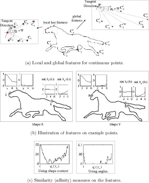
The features and the similarity measure. Panel (a) illustrates how the local and global features are measured for the complete-contour representation. The left window shows the angles computed at the local neighboring points which are used to compute the local shape features. The right window shows the angles computed in larger neighborhoods to compute the global features. Panel (b) displays the features of two points in shape X and Y. As angles have periodic property, we show the a angle vectors by their sinusoid values. As we can see, the corresponding points i on X and a on Y, and k on X and b on Y have similar features. The left and right figure in panel (c) plot the similarities between point a on Y with respect to all points in X using the shape context (on sparse points) feature and angle features (on complete-contour) respectively. As we can see similarities by features defined in this paper for connected points have lower entropy than these given by shape contexts. They are less ambiguous and more informative.

Fig. 3.

The distribution p(θ|X, Y), shown in (f), has three modes for a target shape X, shown in (a), and a source shape Y, shown in (b). The three possible values for θ are shown in (c), (d), and (e).

Fig. 4.

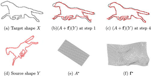
The dynamics of the algorithm for the horse example.

Fig. 5.

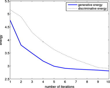
Illustration of the decrease of generative free energy and discriminative free energy by our algorithm. We see that both the free energies consistently decrease w.r.t. time.

Fig. 7.

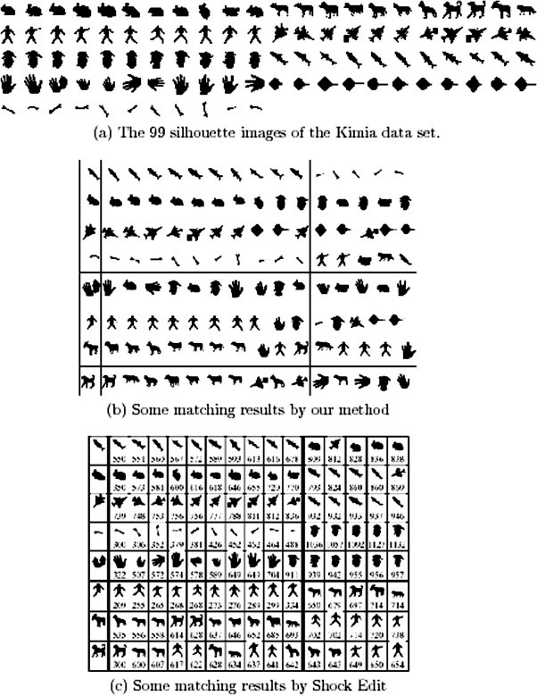
The Kimia data set of 99 shapes and some matching results.

Fig. 8.

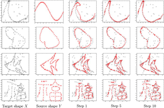
Some results on the Chui and Rangarajan data set.

Fig. 9.

Results on some text images. (c) and (i) display the matching. We purposely superimpose two shapes extracted from different images together and make a new input. Our algorithm is robust in this case.

Fig. 10.

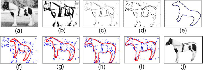
Foreground/background segmentation; (a) input image; (b) the probability map of BEL; (c) the product of BEL map and the canny edge map; (d) sampled points according to the probability (c) ; (e) the template; (f) (i) the result after the first, the third, the 7th and 10th iteration; (j) the segmented foregound according to the matching result.

Fig. 11.

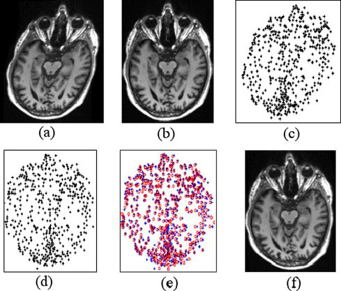
Medical image registration: (a) the unregistered image; (b) the template image; (c) (d) the SIFT key points for the unregistered and template images; (e) the matching result; (f) the registered image.

Fig. 12.

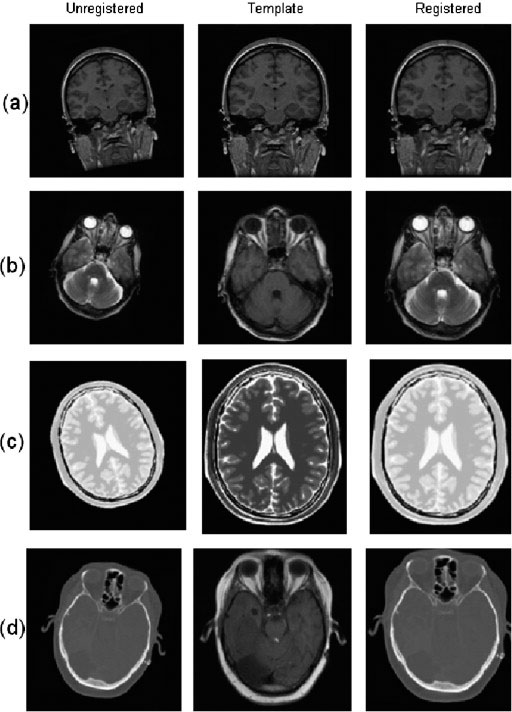
Examples of registration result: (a) MRI registration; (b) registration an unregistered T2 image to a T1 image; (c) registration an unregistered CT image to an MR image; (d) registration an unregistered PD image to a T2 image.

Table 1.

The retrieval rates of different algorithms for the MPEG7 CE-Shape-1. The results by the other algorithms are taken from Sebastian et al. [32].

Algorithm	CSS	Visual Parts	Shape Contexts	Curve Edit Distance	Our Method
Recognition Rate	75.44%	76.45%	76.51%[4]	78.17%[32]	80.03%

Table 2.

The number of matched shapes by the different algorithms. The results by the other algorithms are due to Sebastian et al. [33].

Algorithm	Top 1	Top 2	Top 3	Top 4	Top 5	Top 6	Top 7	Top 8	Top 9	Top 10
Shock Edit	99	99	99	98	98	97	96	95	93	82
Our Method	99	97	99	98	96	96	94	83	75	48
Shape Contexts	97	91	88	85	84	77	75	66	56	37

References

- 1.Abbasi S, Mokhtarian F. Robustness of Shape Similarity Retrieval under Affine Transformation. Proc. of Challenge of Image Retrieval; Newcastle upon Tyne, UK. Feb. 1999. [Google Scholar]
- 2.Ballard DH. Generalizing the Hough Transform to Detect Arbitrary Shapes. Pattern Recognition. 1981;13(2):714–725. [Google Scholar]
- 3.Basri R, Costa L, Geiger D, Jacobs D. Determining The Similarity of Deformable Shapes. Vision Research. 1998;38(15):2365–2385. doi: 10.1016/s0042-6989(98)00043-1. [DOI] [PubMed] [Google Scholar]
- 4.Belongie S, Malik J, Puzicha J. Shape Matching and Object Recognition Using Shape Contexts. IEEE Trans on Pattern Analysis and Machine Intelligence. 2002 Apr;24(24):509–522. doi: 10.1109/TPAMI.2005.220. [DOI] [PubMed] [Google Scholar]
- 5.Bookstein FL. Principal Warps: Thin-Plate Splines and the Decomposition of Deformations. IEEE Trans on Pattern Analysis and Machine Intelligence. 1989;11(6):567–585. [Google Scholar]
- 6.Borenstein E, Sharon E, Ullman S. Combining top-down and bottom-up segmentation. Proc IEEE workshop on Perc Org in Com Vis. 2004 Jun;4:46–53. [Google Scholar]
- 7.Chen X, Yuille AL. AdaBoost Learning for Detecting and Reading Text in City Scenes. Proc. IEEE Conf. Computer Vision and Pattern Recognition; Washington, DC. June 2004.pp. 366–373. [Google Scholar]
- 8.Chui H, Rangarajan A. A New Point Matching Algorithm for Non-rigid Registration. Computer Vision and Image Understanding. 2003 Feb;89:114–141. [Google Scholar]
- 9.Dempster AP, Laird NM, Rubin DB. Maximum-likelihood from Incomplete Data via the Em Algorithm. J Royal Statist Soc, Ser B. 1977;39 [Google Scholar]
- 10.Dollár P, Tu Z, Belongie S. Supervised learning of edges and object boundaries. Proc. IEEE Conf. Computer Vision and Pattern Recognition; New York. June 2006.pp. 1964–1971. [Google Scholar]
- 11.Geiger D, Yuille AL. A common framework for image segmentation. Int’l Journal of Computer Vision. 1991 Aug;6(3):227–243. [Google Scholar]
- 12.Grenander U. General Pattern Theory: A Mathematical Study of Regular Structures. Oxford: 1994. [Google Scholar]
- 13.Helstrom CW. Approximate Evaluation of Detection Probabilities in Radar And Optical Communications. IEEE Trans Aerosp Electron Syst. 2003 July 1;14:630–640. [Google Scholar]
- 14.Hu MK. Visual Pattern Recognition by Moment Invariants. IEEE Trans Inform Theory. 1962;8:179–187. [Google Scholar]
- 15.Keselman Y, Shokoufandeh A, Demirci M, Dickinson S. Many-to-Many Graph Matching via Metric Embedding. Proc. IEEE Conf. Computer Vision and Pattern Recognition; Madison, WI. 2003. pp. 850–857. [Google Scholar]
- 16.Klassen E, Srivastava A, Mio W, Joshi SH. Analysis of Planar Shapes Using Geodesic Paths on Shape Spaces. IEEE Trans on Pattern Analysis and Machine Intelligence. 2004 Mar;26(3):372–383. doi: 10.1109/TPAMI.2004.1262333. [DOI] [PubMed] [Google Scholar]
- 17.Kumar MP, Torr PHS, Zisserman A. OBJCUT. Proc IEEE Conf Computer Vision and Pattern Recognition. 2005;1:18–25. [Google Scholar]
- 18.Latechi LJ, Lakamper R, Eckhardt U. Shape Descriptors for Non-rigid Shapes with a Single Closed Contour. Proc IEEE Conf Computer Vision and Pattern Recognition. 2000 Jun;1:424–429. [Google Scholar]
- 19.Loncaric S. A Survey of Shape Analysis Techniques. Pattern Recognition. 1998 Aug;31(8):983–1001. [Google Scholar]
- 20.Lowe DG. Distinctive Image Features From Scale-invariant Keypoints. Int’l Journal of Computer Vision. 2004;60(2):91–110. [Google Scholar]
- 21.Luo B, Hancock ER. A Unified Framework for Alignment and Correspondence. Computer Vision and Image Understanding. 2003 Oct;92(1):26–55. [Google Scholar]
- 22.Maes F, Collignon A, Vandermeulen D, Marchal G, Suetens P. Multimodality Image Registration by Maximization of Mutual Information. IEEE Trans on Medical Imaging. 1997 Feb;16(2):187–198. doi: 10.1109/42.563664. [DOI] [PubMed] [Google Scholar]
- 23.Maintz JB, Viergever MA. A Survey of Medical Image Registration. Medical Image Analysis. 1998;2(1):1–36. doi: 10.1016/s1361-8415(01)80026-8. [DOI] [PubMed] [Google Scholar]
- 24.Mokhtarian F, Mackworth AK. A Theory of Multiscale, Curvature-Based Shape Representation for Planar Curves. IEEE Trans on Pattern Analysis and Machine Intelligence. 1992 Aug;14(8):789–805. doi: 10.1109/tpami.1986.4767750. [DOI] [PubMed] [Google Scholar]
- 25.Moradi M, Abolmaesoumi P, Mousavi P. Deformable Registration Using Scale Space Keypoints. Medical Imaging 2006: Image Processing Proceedings of the SPIE. 2006;6144:791–798. [Google Scholar]
- 26.Neal R, Hinton GE. Learning in Graphical Models. MIT Press; 1998. A View Of The Em Algorithm That Justifies Incremental, Sparse, And Other Variants; pp. 355–368. [Google Scholar]
- 27.Paragios N, Rousson M, Ramesh V. Matching Distance Functions: A Shape-to-Area Variational Approach for Global-to-Local Registration. Proc of European Conference on Computer Vision. 2002;2:775–788. [Google Scholar]
- 28.Pelillo M, Siddiqi K, Zucker SW. ”Matching Hierarchical Structures Using Association Graphs. IEEE Trans on Pattern Analysis and Machine Intelligence. 1999 Nov;21(11):1105–1119. [Google Scholar]
- 29.Pluim JP, Maintz JBA, Viergever MA. Mutual-information-based Registration of Medical Images: A Survey. IEEE Trans on Medical Imaging. 2003 Aug;22(8):986–1004. doi: 10.1109/TMI.2003.815867. [DOI] [PubMed] [Google Scholar]
- 30.Rangarajan A, Coughlan JM, Yuille AL. A Bayesian Network for Relational Shape Matching. Proc of Int’l Conf on Computer Vision. 2003;1:671–678. Nice France. [Google Scholar]
- 31.Ren X, Fowlkes C, Malik J. Proc of Advances in Neural Information Processing Systems 18. MIT Press; 2005. Cue Integration in Figure/Ground Labeling; pp. 1121–1128. [PubMed] [Google Scholar]
- 32.Sebastian TB, Klein PN, Kimia BB. On Aligning Curves. IEEE Trans on Pattern Analysis and Machine Intelligence. 2003;25(1):116–125. doi: 10.1109/TPAMI.2004.1273924. [DOI] [PubMed] [Google Scholar]
- 33.Sebastian TB, Klein PN, Kimia BB. Recognition of Shapes by Editing their Shock Graphs. IEEE Trans on Pattern Analysis and Machine Intelligence. 2004 May;26(5):550–571. doi: 10.1109/TPAMI.2004.1273924. [DOI] [PubMed] [Google Scholar]
- 34.Sharon E, Mumford D. 2D-Shape Analysis using Conformal Mapping. Proc IEEE Conf Computer Vision and Pattern Recognition. 2004 Jun;2:350–357. [Google Scholar]
- 35.Thayananthan A, Stenger B, Torr PHS, Cipolla R. Shape Context and Chamfer Matching in Cluttered Scenes. Proc IEEE Conf Computer Vision and Pattern Recognition. 2003;1:127–133. [Google Scholar]
- 36.Tu Z, Chen X, Yuille A, Zhu SC. Image Parsing: Unifying Segmentation, Detection and Recognition. Int’l Journal of Computer Vision. 2005 Jul;63(2):113–140. [Google Scholar]
- 37.Tu Z, Yuille A. Shape Matching and Recognition–Using Generative Models and Informative Features. Proc of European Conference on Computer Vision. 2004;III:195–209. [Google Scholar]
- 38.Urschler M, Bauer J, Ditt H, Bischof H. SIFT and Shape Context for Feature-Based Nonlinear Registration of Thoracic CT Images. International ECCV Workshop on Computer Vision Approaches to Medical Image Analysis; Graz, Austria. 2006. pp. 73–84. [Google Scholar]
- 39.Veltkamp RC, Hagedoorn M. Technical Report UU-CS-1999–27. Utrecht; 1999. State of the Art in Shape Matching. [Google Scholar]
- 40.Wells WM, III, Viola P, Atsumi H, Nakajima S, Kikinis R. Multi-modal Volume Registration by Maximization of Mutual Information. Medical Image Analysis. 1996;1(1):35–52. doi: 10.1016/s1361-8415(01)80004-9. [DOI] [PubMed] [Google Scholar]
- 41.Yuille AL, Grzywacz NM. A Computational Theory for the Perception of Coherent Visual Motion. Nature. 1988;333(6168):71–74. doi: 10.1038/333071a0. [DOI] [PubMed] [Google Scholar]
- 42.Yuille AL. Generalized Deformable Models, Statistical Physics, and Matching Problems. Neural Computation. 1990;2(1):1–24. [Google Scholar]
- 43.Zahn CT, Roskies RZ. Fourier Descriptors for Plane Closed Curves. IEEE Trans on Computers. 1972 Mar;C-21(3):269–281. [Google Scholar]
- 44.Zhu SC, Yuille AL. FORMS: A Flexible Object Recognition and Modeling System. Int’l Journal of Computer Vision. 1996;20(3):187–212. [Google Scholar]