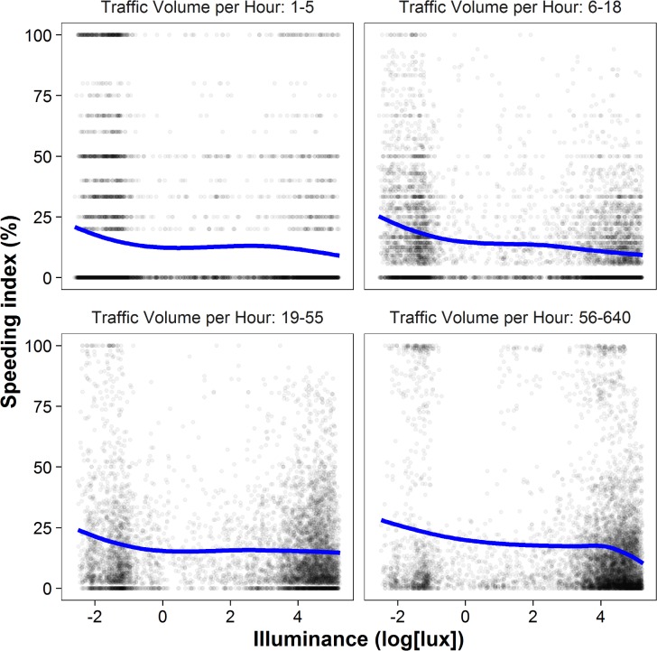
Fig 4. The illuminance‒speeding relationship by traffic volume.

This figure depicts the relationship between illuminance and speeding as in Fig 1, but the data are split by the traffic volume of the respective road per hour. We chose four brackets, each containing a similar number of measurements: 1‒5 vehicles per hour (6497 measurements), 6‒18 (6917), 19‒55 (7012), and 56‒640 (7147). The fitted line shows some variation across the four panels, but they all point to an inverse illuminance‒speeding relationship. Regression analyses for each bracket proved significant: 1‒5 vehicles per hour (b = −0.94, t(6469) = − 7.39, p < .001, partial η² = .01), 6‒18 (b = −1.56, t(6890) = −19.88, p < .001, partial η² = .05), 19‒55 (b = −0.65, t(6985) = −7.65, p < .001, partial η² = .01), and 56‒640 (b = −1.52, t(7116) = −11.85, p < .001, partial η² = .02).