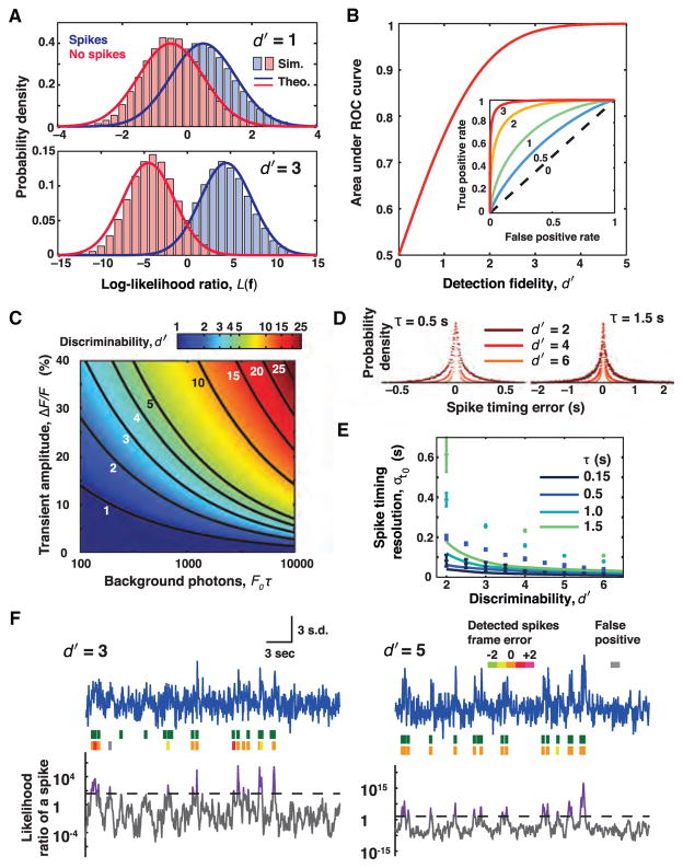
Figure 1. Signal Detection and Estimation Theories Quantify the Physical Limits of Spike Detection Fidelity and Spike Timing Estimation Accuracy in Optical Experiments.

(A) Given a set of photodetector measurements, f, the log-likelihood ratio L(f) quantifies the relative odds that the measurements were of an action potential or not. In general, f can include data from multiple photodetectors or camera pixels and can extend over multiple time bins. Formally, L(f) is a logarithm of a ratio of probabilities, greater than 0 if a neural spike is more likely to have occurred and less than 0 if it is more likely there was no spike. The decision of whether to classify f as representing a spike is enacted by setting a threshold value of L(f); the exact value depends on the experiment’s relative tolerances to false-positive versus false-negative errors. To analyze a full experiment one usually must make multiple classifications of this kind, across each successive time bin, to attain a digitized record of the spike train. Across the subset of all measurements that, in reality, represent the occurrence of a neural spike the mean value of L(f) will be positive (blue data). Across all measurements in which no spike actually occurred, this mean value will be negative (red data). Comparison of the two probability distributions of L(f), one for each of the two hypotheses, allows an assessment of how easy or challenging it is to distinguish the two cases. When the limiting noise source in the experiment is photon shot noise and the non-responsive, baseline photon flux is greater than the signal flux in response to a spike, the distribution of L(f) for each of the two hypotheses is approximately Gaussian. The metric of spike detection fidelity, d′, is the separation in the means of the two Gaussian distributions in units of their standard deviation and describes the degree to which the two hypotheses can be reliably distinguished. The greater the overlap area between the two distributions, the harder on average it is to distinguish if a spike occurred. Distributions of L(f) for d′ = 1 and d′ = 3 are plotted using signal detection theory (solid lines) and from computer simulations of photon statistics (histograms).

(B) One formalizes the decision of whether a spike occurred or not by choosing a threshold value of L(f) to serve as a decision cutoff that allows one to classify individual measurements, f. Inset: Plotting the probability of successful spike detection against the probability of a false alarm for different values of the decision cutoff yields a curve known as the receiver operating characteristic (ROC) curve. Like d′, the area under the ROC curve is a metric of spike detection fidelity that does not depend on the choice of decision threshold. Several ROC curves are plotted, indexed by their d′ values. Main panel: The area under the ROC curve is plotted as a function of the d′ value. Crucially, the area under the ROC curve quickly approaches unity as d′ rises. This is because the overlap in the tails of the two Gaussian L(f) distributions decreases faster than exponentially with increases in d′ (panel A). A non-intuitive but important implication is that modest improvements in d′, which has linear and polynomial relationships to the most common optical parameters, sharply reduce the spike detection error rate. Hence, incremental improvements to indicators, cameras, and other optical hardware can yield huge dividends toward successfully capturing neural activity.

(C) d′ depends on the signal amplitude of the neural activity indicator’s response to an action potential and on the mean number of background photons collected during the indicator’s optical transient. When the Gaussian approximation is valid, and the fluorescence emissions comprise a stationary mean baseline flux, F₀, plus a modest signal transient that arises nearly instantaneously at each spike incidence and then decays exponentially with time constant τ, the expression for d′ reduces to approximately (ΔF/F)·√(F₀τ/2). This shows that indicators with prolonged optical signal transients improve spike detection, since analyses can make use of the signal photons that arrive over the transient’s entire duration. At a constant value of ΔF/F, signal detection improves with increasing background due to the concomitant increase in signal photons.

(D) Simulations of spike timing resolution. Using a brute-force maximum likelihood method for estimating the spike time, histograms of the spike timing error for two indicators with distinct signaling kinetics are shown. Note the different time scales on the two panels. For visual clarity, histograms are normalized to a common peak value. Simulations used 50 ms time bins.

(E) Plots of simulated spike timing resolution and the theoretically calculated Chapman-Robbins lower bound on spike timing estimation errors. The simulations (points) generally do not attain the Chapman-Robbins lower bound (lines), especially for situations with low SNR and slow temporal dynamics. The Chapman-Robbins lower bound should be considered a best-case for estimation variance.

(F) Simulated optical traces and detected spikes for d′ = 3 and d′ = 5. Blue traces: optical measurements shown in units of the standard deviation from the mean photon count. Green spikes: the true spike train. Orange spikes: correctly estimated spikes. Spikes in non-orange hues: spikes estimated with errors in frame timing. Gray spikes: false positives. Gray trace: L(f) for a moving window of nine time bins. Dashed black line: spike detection threshold given equal costs for false positives and false negatives. Purple: threshold crossings. Spikes were detected using an iterative algorithm that assigned a spike to the instance of the log-likelihood ratio’s maximum in each iteration. At low d′, few spikes are detected with this choice of threshold.

All panels are adapted from Wilt et al. (2013).