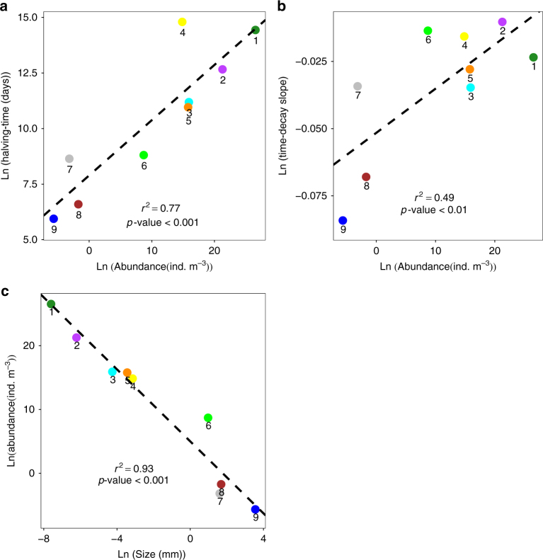
Fig. 3.

Correlations between halving-time and time-decay slopes with local abundance. a Correlation between the logarithms of halving-time (y) and local abundance (x) in main biological groups; linear regression equation y = 7.892 + 0.248x, n = 9, r² = 0.766, p-value <0.001. b Correlation between the logarithms of the time-decay slope (y) and local abundance (x) in main biological groups; linear regression equation y = −0.051 + 0.001x, n = 9, r² = 0.487, p-value <0.01. c Correlation between the logarithms of local abundance (y) and body size (x) in main biological groups; linear regression equation y = 5.002 − 2.820x, n = 9, r² = 0.930, p-value <0.001. Main biological groups: prokaryotes (1); microbial eukaryotes all (2); coccolithophores 0–160 m (3); dinoflagellates 0–160 m (4); diatoms 0–160 m (5); mesozooplankton surface (6); gelatinous zooplankton (7); macrozooplankton (8); myctophids (9). Ln = Napierian logarithm. P-value is calculated at 95% of confidence interval in non-parametric bootstrap cross-validation