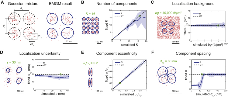
Figure 2.

Evaluation of EMGM using simulated data. (A) On the left is an example of a simulated Gaussian mixture consisting of K = 4 components, each containing 100 localizations, described by a symmetric 2D Gaussian distribution with a SD σ_x = σ_y = 20 nm. The Gaussian centers are placed in a square grid with spacing d_x,y = 100 nm. On the right is the EMGM result. The red dots symbolize the localizations. The blue dots symbolize the center positions and the blue ellipses symbolize the 2σ error ellipses of the components. (B) On the right, the average number of mixture components correctly identified by EMGM as a function of the simulated K. On the left is an example EMGM result for K = 16. (C) On the right is the average SD σ_x,y of the mixture components calculated by EMGM as a function of the simulated localization background density bg. On the left is an example EMGM result for bg = 40,000 #/μm². (D) On the right is the average σ_x,y calculated by EMGM as a function of the simulated localization uncertainty s. On the left is an example EMGM result for s = 30 nm. (E) On the right is the average eccentricity σ_x/σ_y of the mixture components calculated by EMGM as a function of the simulated σ_x/σ_y. On the left is an example EMGM result for σ_x/σ_y = 0.2. (F) On the right is the average number of mixture components correctly identified by EMGM as a function of the simulated spacing d_x,y. On the left is an example EMGM result for d_x,y = 60 nm. The simulated Gaussian mixtures in (C–F) consist of K = 4 components, similar to (A). The dashed lines in (B–F) represent the ground truth, and the shaded areas represent the SD (n = 100).