Assessment of Global and Local Region-based Bilateral Mammographic Feature Asymmetry to Predict Short-Term Breast Cancer Risk

Abstract

This study aims to develop and test a new imaging marker-based short-term breast cancer risk prediction model. An age-matched dataset of 566 screening mammography cases was used. All “prior” images acquired in the two screening series were negative, while in the “current” screening images, 283 cases were positive for cancer and 283 cases remained negative. For each case, two bilateral cranio-caudal view mammograms acquired from the “prior” negative screenings were selected and processed by a computer-aided image processing scheme, which segmented the entire breast area into 9 strip-based local regions, extracted the element regions using difference of Gaussian filters, and computed both global- and local-based bilateral asymmetrical image features. An initial feature pool included 190 features related to the spatial distribution and structural similarity of grayscale values, as well as of the magnitude and phase responses of multidirectional Gabor filters. Next, a short-term breast cancer risk prediction model based on a generalized linear model (GLM) was built using an embedded stepwise regression analysis method to select features and a leave-one-case-out cross-validation method to predict the likelihood of each woman having image-detectable cancer in the next sequential mammography screening. The area under the receiver operating characteristic curve (AUC) values significantly increased from 0.5863±0.0237 to 0.6870±0.0220 when the model trained by the image features extracted from global regions and by features extracted from both the global and the matched local regions(p=0.0001). The odds ratios values monotonically increased from 1.00 to 8.11 with a significantly increasing trend in slope (p=0.0028) as the model-generated risk score increased. In addition, the AUC values were 0.6555±0.0437, 0.6958±0.0290 and 0.7054±0.0529 for the 3 age groups of 37-49, 50-65 and 66-87 years old, respectively. AUC values of 0.6529±0.1100, 0.6820±0.0353, 0.6836±0.0302 and 0.8043±0.1067 were yielded for the 4 mammography density sub-groups (BIRADS from 1 to 4), respectively. This study demonstrated that bilateral asymmetry features extracted from local regions combined with the global region in bilateral negative mammograms could be used as a new imaging marker to assist in the prediction of short-term breast cancer risk.

1. INTRODUCTION

In order to detect breast cancer at an early stage and thus help reduce the mortality rate of breast cancer patients, mammography is the most popular population-based breast cancer screening imaging modality accepted in current clinical practice (Siegelet al. 2013). Interpreting mammograms, however, is a difficult task that requires special training and experience due to the superimposition of breast tissues in mammograms and the low prevalence of cancer (i.e., <0.5%) in a screening population (Casti et al. 2015, Sickles et al. 2002). In addition to the lower detection sensitivity and higher false-positive recall rates of screening mammography (Hubbard et al., 2011), limited healthcare resources and associated high screening costs are also major issues in current breast cancer screening practices (Yaffe and Mainprize 2010, Buist et al. 2011 ). Thus, the efficacy of current mammography screening is quite low and is controversial (Berlin and Hall 2010, Nelson et al. 2009). In order to overcome such limitations, it is desirable to establish more effective personalized screening recommendations based on the assessment of the individualized risk of having or developing breast cancer in the short-term (e.g., < 2 to 5 years) (Brawley 2012), which has recently been attracting significant research interest (Schousboe et al. 2011, Nicolien et al. 2012, Heidi et al. 2012). The goal of these research efforts is to identify a small fraction of women with significantly higher than average short-term risk of developing image-detectable breast cancer. As a result, only those high-risk women should be more frequently screened, while the vast majority of women at average or lower short-term risk of developing cancer can be screened at longer intervals to help increase cancer detection yield and reduce false-positive recalls or unnecessary negative biopsies.

In the breast cancer risk assessment field, a number of breast cancer risk assessment or prediction models e.g., Tyrer-Cuzick, Gail, Claus, and others (Amir et al. 2010, Martin et al. 2010), have been well developed and used. These risk models were primarily developed using several epidemiologically generated risk factors, including the woman’s age, a family history of breast and/or ovarian cancer, breast density, and other life-style factors, to estimate the long-term or lifetime relative risk of having or developing breast cancer in women as compared to the general population risk. However, the risk levels predicted by these models remain constant for an individual woman throughout her lifetime, while cancer development is a progressive process and the short-term breast cancer risk varies with age. Therefore, to identify the probability of women who need to be frequently screened (e.g., annually), a new short-term breast cancer risk prediction model should include the risk factors that produce variable values with a decreasing time lag between negative and positive screenings (Zheng et al. 2014).

For this purpose, quantitative image features or markers can play an important role in detecting or predicting short-term breast cancer risk, since the image features vary with the progression of breast abnormality or cancer development. In an effort to develop image marker-based breast cancer risk prediction schemes or models, several research groups have developed computer-aided detection (CAD) schemes to segment and assess mammographic density as a breast cancer risk prediction marker (Schousboe et al. 2011, Boyd et al. 2011, Li et al. 2014, Pankratz et al. 2015, Li et al. 2012, Heine et al. 2012). Previous studies have also investigated and demonstrated that bilateral mammographic density asymmetry had significantly higher discriminatory power for the prediction of short-term breast cancer risk than the image features computed from single mammograms (Zheng et al. 2012, Tan et al. 2013, 2015, 2016). However, the previous studies only focused on the global bilateral asymmetry of mammographic tissue density-related features. When radiologists read mammograms in clinical practice, bilateral local tissue density asymmetry is often the first important sign attracting their attention to assess cancer risk and detect suspicious lesions (Smith et al. 2016, Boyd et al. 2007). Thus, in this study, we developed and tested a new short-term breast cancer risk prediction model that integrated image features computed from both global and matched local bilateral asymmetry features. The detailed framework of the model and its performance are presented in the following sections of this article.

2. IMAGE DATASET AND METHODS

2.1. The dataset

From a previously established and reported full-field digital mammography (FFDM) image database (Tan et al. 2014), we assembled a unique image dataset of negative mammography screening images. Specifically, we first retrospectively collected all 2500 available cases who have underwent at least two sequential FFDM examinations of both left and right breasts during 2006-2015 in the clinical facilities of university of Pittsburgh medical centre (Zheng et al., 2012). From the results of the latest FFDM examination on record (or namely, the “current” images), 1146 were considered “positive” cases including 1021 screening detected cancer cases, 106 interval cancer cases and 19 high-risk pre-cancer cases with surgically-removed lesion. Among the remaining 1354 “negative” cases, 616 were diagnosed with benign lesions or recalled but later proved to be benign or negative in the additional image workup or biopsy, and 738 were screening negative (not recalled). From this pre-assembled database with 2500 cases, we selected the unique age-matched dataset including 566 cases for this study, in which 283 were developed cancer and the remaining 283 were screening negative (not recall) in the last FFDM examination. Excepted for the last FFDM examination termed as “current” examination, all “prior” examinations in the dataset had been interpreted as “negative” during the originally clinical interpretation and had not been recalled.The mammograms were acquired from 566 women participating in routine mammography screening. All images in this dataset were read and interpreted by radiologists as negative. Then, based on the results of the next sequential (or “current”) mammography screening after 12 to 18 months of these “prior” negative screenings, half of the mammography screening cases (283) were positive, with cancer detected and pathologically verified. The other half (283) remained negative (cancer-free). As a result, we divided 566 negative mammography screening cases into two groups, namely, (1) the high-risk group in which cancer was detected in the next sequential mammography screening and (2) the low-risk group in which the next sequential mammography screening remained negative.

In each group, the women had an age range from 37 to 87 years old. Table 1 presents and compares the distribution of cases in the high- and low-risk groups. The comparison shows that this is an exact age-matched dataset in the two risk groups. There is also no statistically significant difference in mammographic (or breast) density assessed by radiologists based on BIRADS guidelines (P=0.846). Then, for each case, two bilateral cranio-caudal (CC) view mammograms of the left and right breasts were selected and used in this study to develop and test our new short-term breast cancer risk model.

Table 1.

Distribution and comparison of case information in the two risk groups

Risk factor	Category	High-Risk Group	Low-Risk Group	P-value
Age (Years)	Total cases	283	283
	Mean±SD	56.83±9.93	56.83±9.94	0.9933
	<50 years old	76 (26.86%)	76 (26.86%)	1
	50-65 years old	160 (56.54%)	160 (56.54%)	1
	>65 years old	47 (16.61%)	47 (16.61%)	0.9843
Density BIRADS	Almost all fatty tissue (1)	13 (4.59%)	13 (4.59%)	0.8461
	Scattered fibroglandular densities (2)	111 (39.22%)	110 (38.87%)
	Heterogeneously dense (3)	152 (53.71%)	150 (53%)
	Extremely dense (4)	7 (2.47%)	10 (3.53%)

2. 2. METHODS

We developed and tested a number of computer-aided image processing and quantitative image feature analysis algorithms or schemes to detect and quantify both global- and local-based bilateral asymmetry of mammographic features. Figure 1 shows a flow chart of applying our computer-aided detection (CAD) schemes to develop and test our new short-term breast cancer risk prediction model in this study. The detailed methodology of this study is discussed below.

Figure 1.

Flow chart of the procedure for prediction of short-term breast cancer risk using the proposed method

2. 2.1. Mammogram Feature Extraction

After detection of nipple, which served as a reference point, and the breast skin-line using previously developed methods (Casti et al. 2013, 2013), the CAD scheme segmented the global breast region and a number of local regions, which included horizontal strips, vertical strips and DoG (difference of Gaussian) basic element regions. Specifically, the global breast region was derived by extracting the largest rectangles enclosed in the whole breast region, as shown in figure 2(b). For strips, using the nipple location as a central reference point, 9 horizontal strips were segmented in which 4.5 equally spaced segments were located above the nipple and another 4.5 equally spaced segments were located below the nipple, as shown in figure 2 (c). Nine vertical strips were also segmented parallel to the chest wall by dividing the perpendicular line from the nipple to the chest wall into nine equally spaced segments, as shown in figure 2(d). Then, rectangular stripped regions were derived by extracting the largest rectangles enclosed in each segmented strip, as illustrated in figure 2 (e) and (f). DoG basic element regions were segmented with DoG filters and a morphology method. More specifically, after segmentation of the breast area depicted on each image with a CAD scheme (Zheng et al. 2012), a bandpass filter was applied to eliminate high-frequency noise and to suppress regions with local minima in the image. This filter was implemented by convoluting the source image with two Gaussian functions with kernel sizes of 7 and 51 pixels of full-width at half-maximum and taking the difference of the resulting images (Zheng et al., 1995). A binary image was created by a threshold of 100 digital values, which was empirically determined and used in most of the image regions (Zheng et al. 1995). Finally, after applying a morphological opening operation to remove the small isolated regions, the DoG-based element regions were obtained, as shown in figure 2(g).

Figure 2.

Examples of original image and local regions. (a) original image. (b) global region, (c) and (d), horizontal strips and vertical strips. (e) and (f), rectangular strips. (g) DoG basic element regions.

From the segmented regions, the CAD scheme was also used to compute three groups of image features, including spatial variation features, structural similarity features and positional information features, which are discussed below.

1) Spatial variation features

Structural variations among pixel values in a given region of interest can be described by the semi-variogram, which is a descriptor that quantifies the degree of spatial dependence between samples and measures the structure of the spatial influence of a process (Casti et al. 2015). Given M (d) pairs of pixels separated by a distance d, the semi-variogram is defined in equation (1) as:

$$\nu (d)=\frac{1}{2M(d)}{{\sum }_{n=1}^{M(d)}[I(t_{n,0}-t_{n,d})]}^2$$ (1)

where t_n,0 and t_n,d,; n=1,2,…,M(d) are vectors of spatial coordinates (x, y) separated by the lag distance d, and I is the grey level at the given spatial locations.

Following Casti et al 2015, the maximum value of d, d_max, was set as equal to one-half of the maximum distance between pairs of pixels in each region. Then, the range of distances from 0 to d_max was divided into 20 equally spaced bins and the pixel pairs were aggregated accordingly to estimate the empirical semi-variogram (ν_m) for representative distances of each aggregate. Finally, a least-square fitting of each vm was performed with a spherical structure function, as shown in equation (2):

$$\widehat{\nu }(d)=\{\begin{array}{ll}a+c(\frac{3d}{2r}-\frac{d^3}{2r^3}),& \mathit{if}d\le r\\ a+c,& \mathit{if}d>r\end{array}$$ (2)

where a, the nugget, that gives the discontinuity at the origin; c, the sill, represents an estimate of the variance of pixels; and r, the range of influence of the spatial structure (Casti et al. 2015).

For each strip, we first computed three parameters, including the nugget, sill and range. Then, nine absolute differences for each parameter value were computed from the matched strips of the left and right mammograms. Next, four statistical characteristics for each parameter, including the maximum, median, coefficient of variance (CV) and kurtosis, were both computed from the bilateral matched horizontal and vertical strips. Thus, for each case, the CAD scheme initially computed a total of 72 spatial variation-based bilateral asymmetry features of grayscale values, as well as of the magnitude and phase responses of multidirectional Gabor filters that have been shown to be effective in detecting mammographic asymmetry and architectural distortion (Ferrari et al. 2001, Rangayyan et al. 2007, Banik et al. 2011).We also computed 18 spatial variation-based bilateral asymmetry features for the global region in the horizontal and vertical direction for grayscale values, as well as for the magnitude and phase responses of multidirectional Gabor filters for each case.

2) Structural similarity features

Since structural similarity provides a reasonable approximation of the human visual system, which is adapted for extracting structural information from a particular scene (Rangayyan et al. 2007), we used the SSIM index to access the bilateral asymmetry of mammograms to predict the short-term risk of developing breast cancer. Given a pair of matched right and left rectangular regions, x_R= s{x_i∣i=1,…,M} and y_L ={y_i∣i=1,…,M}, the SSIM index is computed as shown in following equation (3):

$$S(x_R,y_L)=\frac{(2{\mu }_x{\mu }_y+C_1)(2{\sigma }_{\mathit{xy}}+C_2)}{({\mu }_x^2+{\mu }_y^2+C_1)({\sigma }_x^2+{\sigma }_y^2+C_2)}$$ (3)

where ${\mu }_x=\raisebox{1ex}{$1$}\!\left/ \!\raisebox{-1ex}{$M$}\right.{\sum }_{i=1}^M{x}_i,{\sigma }_x^2=\raisebox{1ex}{$1$}\!\left/ \!\raisebox{-1ex}{$M$}\right.{\sum }_{i=1}^M{(x_i-{\mu }_x)}^2,{\sigma }_{\mathit{xy}}=\raisebox{1ex}{$1$}\!\left/ \!\raisebox{-1ex}{$M$}\right.{\sum }_{i=1}^M(x_i-{\mu }_x)(y_i-{\mu }_y)$, C₁ and C₂ are two small positive constants: they were set to 0.01 and 0.03, respectively, to avoid instability when ${\mu }_x^2+{\mu }_y^2$ and ${\sigma }_x^2+{\sigma }_y^2$ is very close to zero, as indicated in the work by Wang et al. 2004. The maximum SSIM index value is 1 and is achieved if and only if x and y are identical (Rangayyan et al. 2007, Banik et al. 2011).

Recently, Casti et al. 2015 presented a Correlation-Based SSIM (CB-SSIM) index that enables direct estimation of structural similarity between regions of different sizes and showed that the CB-SSIM index had the potential to effectively detect bilateral asymmetry through quantification of structural similarity between paired mammogram regions (Tan et al. 2016). As Wang et al. 2004 defined the structural information in an image as three attributes including luminance comparison, contrast comparison and structure comparison. Given a pair of right and left rectangular regions, x_R and y_L, of size M × N and S × T pixels, respectively, the luminance comparison is defined in equation (4) as:

$$l(x_R,y_L)=\frac{2{\mu }_R{\mu }_L+K_1}{{\mu }_R^2{\mu }_L^2+K_1}$$ (4)

where μ_R and μ_L are the mean values of pixels within the right and left regions, respectively, the constant K1 is included to avoid instability when ${\mu }_R^2{\mu }_L^2$ is very close to zero. Similar considerations were also applied to structure comparison and contrast described later. The structure comparison function is defined in equation (5) as

$$s(x_R,y_L)=\frac{\{2\max [\mathit{corr}(x_R,y_L)]+K_2\}}{\max [\mathit{corr}(x_R,x_R)]·\max [\mathit{corr}(y_L,y_L)]+K_2}$$ (5)

where $\mathit{corr}(x_R,y_L)={\sum }_{m=1}^M{\sum }_{n=1}^N\{[x_R(m,n)-{\mu }_R][y_L(m-s,n-t)-{\mu }_L]\}$ with -S + 1 ≤ s ≤ M − 1 and −T + 1 ≤ t ≤ N − 1 is cross-correlation between the right and left regions; corr (x_R, x_R) and corr (y_L, y_L) are the corresponding auto-correlation functions. The constant K₂ is included to avoid instability when max[corr (x_R, x_R)] · max[ corr (y_L , y_L)] very close to zero. The contrast comparison function takes a similar form as shown in equation (6)

$$c(x_R,y_L)=\frac{\{2\max [\mathit{corr}(x_R,x_R)]·\max [\mathit{corr}(y_L,y_L)]+K_3\}}{\max [\mathit{corr}(x_R,x_R)]+\max [\mathit{corr}(y_L,y_L)]}$$ (6)

where K₃ is a small constant. Finally, we combined the three comparisons of (4), (5) and (6) with the equal relative importance of the three components and K₃ was set equal to 2K₂ as indicated in the work by Wang et al. 2004. As a specific form of the CB-SSIM index is shown in equation (7)

$${\stackrel{\sim }{S}}_{(x_R,y_L)}=\frac{(2{\mu }_R{\mu }_L+K_1)\{2\max [\mathit{corr}(x_R,y_L)]+K_2\}}{({\mu }_R^2{\mu }_L^2+K_1)\{\max [\mathit{corr}(x_R,x_R)]+\max [\mathit{corr}(y_L,y_L)]\}}$$ (7)

The “universal quality index” corresponds to the special case that K₁=K₂=0, which produces unstable results when either ${\mu }_R^2{\mu }_L^2$ or max[corr (x_R, x_R)] · max[corr (y_L, y_L)] is very close to zero. ConstantK₁ and K₂ were set to 0.01 and 0.03 respectively, as indicated in the work by Casti et al. 2015.

Since the sizes of the 2 matched strips extracted from two bilateral images are typically not equal, we aligned 2 strips by registering their centers and used a smaller region as a reference to generate 2 strips of the same size by eliminating the pixels outside the overlapped regions (Tan et al. 2016). The SSIM index was then computed for each matched strip of an equal size. The CB-SSIM index was estimated directly between 2 different-sized bilateral regions. Thus, nine SSIM index values and nine CB-SSIM index values were both computed for the horizontal and vertical strips for each case. Next, two statistical characteristics, the range and mean deviation of the SSIM and CBSSIM indices, were computed for both the horizontal and vertical strips as bilateral asymmetry features to assess short-term breast cancer risk. Thus, in this group, CAD initially computed 24 features related to the structural similarity of image grayscale values as well as of the magnitude and phase responses of multidirectional Gabor filters for each case. In addition, CAD also computed 6 structural similarity-related bilateral asymmetry features from the global breast region in grayscale values and magnitude and phase responses of multidirectional Gabor filters for each case.

3) Position information features

Since a DoG filter is usually used to identify the initial set of suspicious regions in mammograms (Catarious et al. 2006), which reflect details of intensity variations in breast tissue (Rafiee et al. 2013), we analysed the position information of DoG basic element regions to assess bilateral asymmetry between the left and right breasts for prediction of short-term breast cancer risk in this study. After DOG basic element regions were generated, we established a coordinate system in which the nipple position serves as origin of the system, and two lines that are perpendicular and parallel to the chest wall serve as the x and y axis, respectively, as illustrated in figure 3(a).

Figure 3.

Examples of the coordinate system and six sub-regions. (a) Coordinate system. (b) Six sub-regions.

Next, two position parameters, the distance ρ and the angle θ, between the nipple and the coordinates (x, y) of the pixel from DoG-based element regions were computed. Five statistical characteristics (sum, median, maximum, minimum and standard deviation) for each parameter value were computed. Then, the absolute difference values for five statistical characteristics between left and right mammograms were computed, both for distance and angle as bilateral asymmetry features to predict short-term breast cancer risk. As a result, we computed a total of 10 positional features for DoG basic element regions spread over the whole breast region for each case.

In addition, instead of dividing 9 horizontal and 9 vertical strip sub-regions, we divided the whole breast region into six sub-regions and computed positional features for each sub-region, which may provide more accurate bilateral asymmetry. Specifically, 3 horizontal regions were first segmented in which 1.5 equally spaced segments were located above the nipple and another 1.5 equally spaced segments were located below the nipple. Two equally spaced vertical regions were segmented parallel to the chest wall by dividing the perpendicular line from the nipple to the chest wall into 2 equally spaced segments. Thus, six sub-regions were segmented, as shown in figure 3 (b). The same position features as described above were extracted from DoG basic element regions spread over each sub-region. Thus, 60 positional-based bilateral asymmetry features for DoG basic element regions spread over six sub-regions were computed for each case.

2. 2.2 Feature Analysis and Performance Assessment

After an initial 190 bilateral mammographic tissue density asymmetry features were computed from the left and right CC view mammograms, we trained a generalized linear model (GLM)-based machine learning classifier using an embedded feature selection and a leave-one-case-out (LOCO) validation method to maximally use all available training cases and also minimize the testing bias (Li and Doi 2006). In each LOCO training and testing cycle, we first applied a standard step-wise regression-based feature selection method (Tan et al. 2016, Häberle et al. 2012) to automatically select a set of “effective” and/or “relevant” image features from the initial feature pool of 190 features reported in Sec. 2.B.1. This step eliminated redundant image features and reduced the curse of dimensionality or the risk of “overfitting” the classifier during the training procedure. This feature selection process was embedded within each LOCO-based cross-validation cycle to avoid case selection bias during the GLM optimization task (Varma and Simon 2006).A step-wise regression method was applied to select a set of optimal features and build a GLM classifier. The classifier was then applied to one remaining testing case to generate a risk prediction score. This process was iteratively executed until all 566 cases in our dataset were tested. Basically, using this LOCO training and testing process, 566 different GLM classifiers were built and tested, which may use different features and have different weights or parameters used in the model. As a result, each case has a GLM-generated risk score. A higher score indicates a higher risk or likelihood of having a mammography-detectable breast cancer during the “current” examination.

Next, we used the area under the receiver operating characteristic (ROC) curve (AUC), which was computed using a publicly available maximum likelihood-based ROC curve fitting program (ROCKIT, http://www-radiology.uchicago.ed/krl/, University of Chicago), as an evaluation index to assess the performance of applying the image features and/or the GLM classifier-generated risk prediction scores to predict short-term breast cancer risk, which means the likelihood of a woman having image-detectable cancer in the next sequential mammography screening in this study. The adjusted odds ratios (ORs) were also calculated based on a multivariate statistical model using a statistical software package (R version 3.4.0, http://www.r-project.org). A possible OR increasing trend with increasing risk prediction scores was then computed and analysed.

We also performed a number of additional studies. First, in addition to analysing the trend of the risk score generated by the risk model in all cases, we also analysed the trend of the risk prediction performance in 3 age-based sub-groups. For this purpose, we computed and compared AUC values for 3 age-based sub-groups with the risk score generated by the risk model as described above. Second, we computed and analysed the trend of the risk score generated by the risk model in four sub-groups of cases divided by mammography density originally rated by radiologists based on BIRADS categories. For this purpose, we computed and compared AUC values and OR trends for 4 BIRADS-based sub-groups with the risk scores generated by our CAD scheme.

3. RESULTS

Figure 4 compares 3 ROC curves computed using the GLM-generated risk scores for features extracted from both local and global regions, local regions and global regions only, respectively.

Figure 4.

Three ROC curves for application of GLM models to features extracted from the matched local, global and both from local and global regions.

The corresponding AUC values and 95% CIs are shown in Table 2. The image features selected in more than 50% of 566 LOCO cross-validation runs are listed in Table 3. The AUC values are 0.5868±0.0238 and 0.6368±0.0232 when using image features extracted and computed from the global breast regions and the matched local regions, respectively. A combination of features computed from both global and matched local regions yielded the AUC value of 0.6870±0.0220. Table 3 also shows that a total of 11 and 6 image features were selected with more than 50% frequency in 566 LOCO iterations from the matched local and global regions, respectively.

Table 2.

AUC values (standard error, SE) of classifiers applying the GLM-based risk models for features extracted from the matched local and global regions.

Features	AUC (SE)	95% CI
Extracted both from local and global regions	0.6870 (0.0220)	(0.6428, 0.7287)
Extracted from local regions	0.6308 (0.0231)	(0.5848, 0.6750)
Extracted from global regions	0.5863 (0.0237)	(0.5394, 0.6320)

Table 3.

List of features that were selected in more than 50% of the cross validation runs from local and global regions.

Local Feature	Description	Percentage	Local Feature	Description	Percentage	Global Feature	Description	Percentage
F1	coefficient of variance of $r_M^H$	100% (566/566)	F7	range of $S_M^V$	100% (566/566)	F1	$c_G^V$	69.96% (396/566)
F2	kurtosis of $r_M^H$	100% (566/566)	F8	median of ρ3	98.06% (555/566)	F2	sum of ρ0	100% (566/566)
F3	max of $a_G^V$	100% (566/566)	F9	standard deviation of ρ4	100% (566/566)	F3	max of ρ0	99.82%(565/566)
F4	max of $a_P^V$	63.43% (359/566)	F10	max of θ6	99.47% (563/566)	F4	SP	100% (566/566)
F5	median of $r_P^V$	100% (566/566)	F11	min of θ6	99.47% (563/566)	F5	~ SG	96.64%(547/566)
F6	mean deviation of $S_P^H$	98.06% (555/566)	—	—		F6	~ SP	100% (566/566)

Note. a, c, and r: semivariogram descriptors that stand for nugget, sill and range, respectively. S and ŝ : structural similarity descriptors that stand for Structural Similarity index and Correlation-Based Structural Similarity index, respectively. ρ and θ : position information descriptors, namely distance and angle, respectively. H and V: horizontal masking/direction and vertical masking/direction, respectively. G, M and P: grayscale values, the magnitude and phase responses of multidirectional Gabor filters, respectively. 0-6: 0 indicates DoG basic element regions spread over the whole breast region, 1-6 indicate DoG basic element regions spread over the first sub-region to the 6^th sub-region. For example, $r_M^H$ indicates the range from the magnitude of Gabor filters for horizontal strips; Ŝ_G stands for the CB-SSIM index from grayscale values; and ρ₃ stands for the radius of DoG basic element regions spread over the 3rd sub-region.

Table 4 summarizes the adjusted ORs and the corresponding 95% CIs for 5 bins (sub-groups) of cases using the risk prediction scores generated by 3 GLM-based risk models trained using both local and global region features, local region features and global region features only. The classifier-generated risk scores gradually increase from 1 to 5. Using the cases in bin 1 as a baseline, ORs and 95% CIs in bin 2 to 5 were computed and compared. The results demonstrate 3 increasing trends in OR values as a function of increased risk score. The results show that ORs increased from 1.00 in bin 1 to 8.11 in bin 5 (with 95% CI of [4.49, 14.68]) when applying the GLM-based risk models to features extracted both from local and global regions.

Table 4.

Adjusted odds ratios (ORs) and 95% confidence intervals (CIs) for 5 bins with increasing levels of GLM-generated risk scores

Bins	Local and global regions			Local regions			Global regions
	P and N casesa	OR	95% CI	P and N casesa	OR	95% CI	P and N casesa	OR	95% CI
1	29-84	1	Baseline	37-76	1	Baseline	47-66	1	Baseline
2	49-64	2.22	[1.26, 3.89]	53-60	1.81	[1.06, 3.11]	46-67	0.96	[0.57, 0.64]
3	52-61	2.47	[1.41,4.33]	50-63	1.63	[0.95, 2.80]	61-52	1.65	[0.97, 2.79]
4	69-44	4.54	[2.58,8.01]	68-45	3.10	[1.80, 5.35]	60-53	1.59	[0.94, 2.69]
5	84-30	8.11	[4.49,14.68]	75-39	3.95	[2.28, 6.86]	69-45	2.15	[1.27, 3.66]
Pb	0.0028			0.0117			0.0229

^aNumber of P (cancer) and N (cancer-free) cases in the corresponding bin of cases.

^bP-value to analyse whether the slope of the regression trend line between the risk scores and the adjusted ORs is significantly different from zero.

In addition, figure 5 shows that all the regression slopes (trend lines) between the risk prediction scores and the adjusted ORs are significantly different from zero (p<0.05), which also indicates an increasing trend between the risk prediction score generated by the risk models and the actual risk of women having mammography-detectable breast cancer during the “following” screening cycles.

Figure 5.

Increasing trend in the odds ratios with the increase in risk scores for both local and global features, local features and global features.

Table 5 shows the confusion matrix obtained by applying an operational threshold of 0.7 to the risk prediction score of the model generated using features extracted from both local and global regions. At this operational threshold, the overall prediction accuracy of the risk models was 64.31%; that is, 364 of the 566 cases were correctly classified, while 35.69% (202/566) cases were misclassified, which corresponds to a 58.66% (166/283) prediction “sensitivity” at a 69.97% (198/283) prediction “specificity”. The positive predictive value (PPV) of the risk model was 66.14% (166/251), and the negative predictive value (NPV) was 62.86% (198/315).

Table 5.

A confusion matrix obtained for classifier-generated risk/probability scores.

Total population	Condition positive	Condition negative
Predicted condition positive	166	85
Predicted condition negative	117	198

Figure 6 displays and compares 3 ROC curves computed by applying the classifier-generated risk scores to three sub-groups of cases divided by age. The corresponding AUC values are 0.6555±0.0437, 0.6958±0.0290 and 0.7054±0.0529 for sub-groups of 37-49, 50-65 and 66-87 years old, respectively.

Figure 6.

Comparison of three ROC curves in three age-based sub-groups

In addition, figure 7 displays and compares 4 ROC curves applying our risk prediction classifier to four sub-groups of cases divided by mammographic density BIRADS categories. Note that the performance level of BIRADS 2 and BIRADS 3 is very similar and that the ROC curves are nearly overlapping, as shown in Fig. 7. The AUC values are 0.6820±0.0353 and 0.6836±0.0302 for the BIRADS 2 and 3 sub-groups, respectively, while the AUC values increased to 0.8043±0.1067 for BIRADS 4 and decreased to 0.6529±0.1100 for BIRADS 1, which are not reliable due to the small number of cases in these two BIRADS categories (as shown in Table 1).

Figure 7.

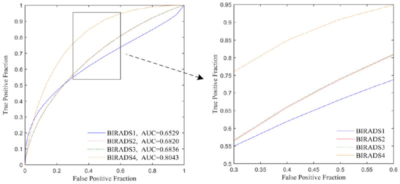
Four ROC curves in four BIRADS-based sub-groups. ROC curves of BIRADS 2 and BIRADS 3 were almost overlapping. P value is 0.8476 with DeLong’s test for two ROC curves of BIRADS 2 and BIRADS 3.

Table 6 shows and compares the adjusted odds ratios in the mammographic density BIRADS 2 and 3 sub-groups. In both sub-groups, an increasing trend between the model-generated risk scores and the women having mammography-detectable cancer in the next sequential screening is detected with p<0.05. The maximum relative odds ratio is higher in the BIRADS 3 category than in the BIRADS 2 category.

Table 6.

Adjusted ORs for 5 bins in the BIRADS 2 and BIRADS 3 sub-groups

	BIRADS 2			BIRADS 3
Bins	P and N casesa	BIRADS 2 Adjusted OR	95% CI	P and N casesa	BIRADS 3 Adjusted OR	95% CI
1	12-32	1	Baseline	15-45	1	Baseline
2	17-27	1.68	[0.68, 4.13]	28-32	2.63	[1.21, 5.69]
3	22-22	2.67	[1.10, 6.48]	28-32	2.63	[1.21, 5.69]
4	30-14	5.71	[2.28, 14.31]	34-26	3.92	[1.81, 8.52]
5	30-15	5.33	[2.15, 13.22]	47-15	9.4	[4.12, 21.43]
P-value		0.0072b			0.0117b

^aNumber of P (cancer) and N (cancer-free) cases in the corresponding sub-group of cases.

^bP-value to analyse whether the slope of the regression trend line between the risk sores and the adjusted ORs is significantly different from zero.

4. DISCUSSION

Although bilateral mammographic density asymmetry has been previously investigated as a possible short-term breast cancer risk factor (Zheng et al. 2012, Tan et al. 2013, 2015, 2016), accurately detecting bilateral mammographic density asymmetric patterns and computing the effective image features remain a challenging problem. In order to address and overcome this challenge, we investigated a new approach and demonstrated the feasibility and advantages of this new approach. Compared to previous studies in this field, this work has several unique characteristics and yielded a number of research study results or observations. First, although previous studies have investigated and indicated that the image features related to bilateral mammographic density asymmetry had significantly higher discriminatory power for the prediction of short-term breast cancer risk than the image features computed from single mammograms (Zhenget al. 2012, Tan et al. 2013, 2015, 2016), previous studies only focused on detecting and computing the features related to the global bilateral asymmetry of mammographic tissue density. However, when radiologists read mammograms in clinical practice, bilateral local tissue density asymmetry often is the first important sign attracting their attention to assess cancer risk and detect suspicious lesions (Smithet al. 2016, Boyd et al. 2007). In this study, we developed and tested a computer-aided image processing scheme to detect and compute the related image features from both global and the matched local (or regional) bilateral asymmetry of mammographic density features. Then, we built and tested several new risk models using different combinations of the features. Our study results are consistent with how radiologists read and interpret mammograms in clinical practice, which indicates that using the matched local bilateral mammographic features yielded a higher performance than using the model developed based on the bilateral asymmetry of global mammographic image features (AUC=0.5868±0.0238 versus AUC = 0.6368±0.0232). The study also showed that image features extracted from global and matched local regions are complementary (not highly correlated). As a result, a new GLM-based risk model or classifier trained using features combining both global and matched local features yielded a significantly improved risk prediction performance of AUC = 0.6870±0.0220 compared to the results obtained using the risk prediction scores generated using the models trained by the image features extracted separately from local or global regions (P<0.05). It also shows an increasing trend in odds ratios (with a maximum adjusted OR of 8.11) of short-term cancer risk with the increase in model-generated risk scores.

Second, since the performance of any breast cancer risk prediction model depends on the different training and testing datasets, we are unable to directly compare the performance of this study with many of the previously reported studies due to the use of different image datasets. However, unlike many previous studies in this field (e.g.,Zhenget al. 2012, Tan et al. 2013, 2015, 2016), we used an age-matched dataset involving 566 FFDM cases. Using an age-matched dataset could reduce data analysis bias from age difference or imbalance in the groups of high- and low-risk cases because age is one of the strongest breast cancer risk indicators in many existing breast cancer risk models (Martin et al., 2010). In addition, we built a unique generalized linear model (GLM) using an embedded stepwise regression feature selection method and a LOCO validation method. This approach helps to further reduce two important biases related to the feature and test case selection. Hence, by taking these steps, the results of our study might be more reliable and robust.

Third, unlike previous studies, which primarily focused on computing and analysing the bilateral asymmetry of mammographic tissue density-related features, we analysed a number of new types of features, which include the spatial variation-related features, structural similarity between the right and left mammograms, and position information based bilateral asymmetry features. The information about the spatial dependency of pixels within each mammographic region is extracted by characteristics of spherical semivariogram descriptors, i.e., the nugget, sill, and range, which possess the ability to measure the spatial influence of a process in a given area (Casti et al. 2015). The characteristics of the structural similarity (SSIM) index and correlation-based SSIM (CBSSIM) index are used in this study to derive correlation-based similarity indices for quantification of changes in the structural information of each mammographic region with respect to the corresponding contralateral region. These indices are used to emulate the radiologist’s perception of distortions in mammograms and to improve the accuracy of detecting bilateral asymmetry. In addition, the directional components of breast tissue patterns and the use of Gabor filters for directional analysis have been shown to be effective in detecting mammographic signs of asymmetry and architectural distortion (Ferrari et al. 2001, Rangayyan et al. 2007, Banik et al. 2011). For this reason, the magnitude and phase responses of multidirectional Gabor filters were used in this study, together with the original grayscale values to characterize the structural information of breast parenchyma. At the same time, the difference of Gaussian filters were usually used to detect suspicious regions in mammograms (Rafiee et al. 2013), which reflect details of intensity variations in breast tissue (Catarious et al. 2006). Therefore, characteristics of position information from DoG basic element regions were also extracted for this intended purpose.

Fourth, we observed the performance when applying our risk prediction model to the three age-based sub-groups. The AUC values were 0.6555 ± 0.0437, 0.6958 ± 0.0290 and 0.7054 ± 0.0529 for the sub-groups with an age of 37-49, 50-65 and 66-87 years old. An increasing trend was observed from young to old screening data. This observation may indicate that the variation in mammographic tissue patterns from the negative to positive screening is in concert with age-based cases.

Last, our data analysis for the two sub-groups of cases divided by mammographic density BIRADS categories 2 and 3 showed very similar performance levels (AUC values of 0.6820±0.0353 and 0.6836±0.0302, respectively). The results indicated that although mammographic density assessed using BIRADS is considered an important breast cancer risk factor in many previously reported breast cancer risk models, the model developed here based on computed bilateral mammographic density asymmetry is very different from the mammographic density assessed using BIRADS. The short-term breast cancer risk depends more on the bilateral mammographic density asymmetry rather than the overall or average mammographic density (BIRADS categories).

Although this study demonstrated a promising result, this study also has a number of limitations. First, this is a laboratory-type retrospective study with a relatively small dataset that may involve potential case selection bias and cannot fully represent the diversity in the general breast cancer screening population. Second, we only tracked the detection status change between the two sequential mammographic screening examinations in which the first examination of interest was not retrospectively reassessed in this study. Thirdly, the accuracy of the model prediction is low, which needs to further improve the model performance to enhance the accuracy of prediction. Even though the risk prediction model developed in this study achieved higher near-term breast cancer risk prediction accuracy by combining local and global region based bilateral image features compared to the previous global region based risk models (e.g., Tan et al., 2016) , the AUCs are still not higher enough for use in clinical practice (Gail et al., 2010). And therefore further studies to combine more image features (e.g. more views and modalities) and/or integrate non-image risk factors (such as genetic or demograhic risk factors) are needed to improve risk prediction performance (Zheng et al., 2012). Hence, the risk factor or model developed in this study has only been tested as an attempt to identify women with a significantly higher risk of having breast cancers in the next sequential examination regardless of whether the cancer has been missed or overlooked in the prior “negative” examinations. Therefore, this breast cancer risk model needs to be further examined and validated using larger and more diverse databases in further prospective studies.

5. CONCLUSION

In this study, we presented a novel short-term breast cancer risk prediction scheme based on the combination of both global and localregionbased bilateral asymmetry features in mammography with a machine learning classifier to predict short-term breast cancer risk. To eliminate age bias, which is one of the strongest breast cancer risk indicators, we tested our new risk model using an age-matched image dataset. The performance of this study demonstrated that the new approach we proposed had the potential to develop a new quantitative imaging-based risk model to assist in the prediction of short-term risk for developing breast cancer and thus eventually establish an optimal personalized breast cancer screening paradigm. For this purpose, more effort in development, optimization and evaluation of this short-term breast cancer risk prediction performance is needed in future studies.

References

- Amir E, Freedman OC, Seruga B. Assessing women at high risk of breast cancer: a review of risk assessment models. Journal of the National Cancer Institute. 2010;102:680–691. doi: 10.1093/jnci/djq088. [DOI] [PubMed] [Google Scholar]
- Banik S, Rangayyan RM, Desautels JE. Detection of Architectural Distortion in Prior Mammograms. IEEE Transactions on Medical Imaging. 2011;30:279–294. doi: 10.1109/TMI.2010.2076828. [DOI] [PubMed] [Google Scholar]
- Berlin L, Hall FM. More mammography muddle: emotions, politics, science, costs, and polarization. Radiology. 2010;255:311–316. doi: 10.1148/radiol.10100056. [DOI] [PubMed] [Google Scholar]
- Boyd NF, Martin LJ, Yaffe MJ, Minkin S. Mammographic density and breast cancer risk: current understanding and future prospects. Breast Cancer Research. 2011;13:223. doi: 10.1186/bcr2942. [DOI] [PMC free article] [PubMed] [Google Scholar]
- Boyd NF, et al. Mammographic Density and the Risk and Detection of Breast Cancer. New England Journal of Medicine. 2007;356:227–36. doi: 10.1056/NEJMoa062790. [DOI] [PubMed] [Google Scholar]
- Brawley OW. Risk-based mammography screening: an effort to maximize the benefits and minimize the harms. Annals of Internal Medicine. 2012;156:662–663. doi: 10.7326/0003-4819-156-9-201205010-00012. [DOI] [PubMed] [Google Scholar]
- Buist DS, et al. Influence of annual interpretive volume on screening mammography performance in the United States. Radiology. 2011;259:72–84. doi: 10.1148/radiol.10101698. [DOI] [PMC free article] [PubMed] [Google Scholar]
- Casti P, Mencattini A, Salmeri M, Ancona A, Mangieri FF, Pepe ML, Rangayyan RM. Automatic detection of the nipple in screen-film and full-field digital mammograms using a novel Hessian-based method. Journal of Digital Imaging. 2013;26:948–957. doi: 10.1007/s10278-013-9587-6. [DOI] [PMC free article] [PubMed] [Google Scholar]
- Casti P, Mencattini A, Salmeri M, Ancona A, Mangeri F, Pepe ML, Rangayyan RM. Estimation of the breast skin-line in mammograms using multidirectional Gabor filters-Computers in Biology and Medicine. Computers in Biology & Medicine. 2013;43:1870–1881. doi: 10.1016/j.compbiomed.2013.09.001. [DOI] [PubMed] [Google Scholar]
- Casti P, Mencattini A, Salmeri M, Rangayyan RM. Analysis of Structural Similarity in Mammograms for Detection of Bilateral Asymmetry. IEEE Transactions on Medical Imaging. 2015;34:662–671. doi: 10.1109/TMI.2014.2365436. [DOI] [PubMed] [Google Scholar]
- Catarious DM, Baydush AH, Floyd CE. Characterization of difference of Gaussian filters in the detection of mammographic regions. Medical Physics. 2006;33:4104–4114. doi: 10.1118/1.2358326. [DOI] [PubMed] [Google Scholar]
- Ferrari RJ, Rangayyan RM, Desautels JE, Frere AF. Analysis of asymmetry in mammograms via directional filtering with Gabor wavelets. IEEE Transactions on Medical Imaging. 2001;20:953–964. doi: 10.1109/42.952732. [DOI] [PubMed] [Google Scholar]
- Gail MH, Mai PL. Comparing breast cancer risk assessment models. J Natl Cancer Inst. 2010;102:665–668. doi: 10.1093/jnci/djq141. [DOI] [PubMed] [Google Scholar]
- Häberle L, et al. Characterizing mammographic images by using generic texture features. Breast Cancer Research. 2012;14:1–12. doi: 10.1186/bcr3163. [DOI] [PMC free article] [PubMed] [Google Scholar]
- Nelson Heidi D, et al. Risk factors for breast cancer for women aged 40 to 49 years: a systematic review and meta-analysis. Annals of Internal Medicine. 2012;156:635–648. doi: 10.1059/0003-4819-156-9-201205010-00006. [DOI] [PMC free article] [PubMed] [Google Scholar]
- Heine JJ, et al. A Novel Automated Mammographic Density Measure and Breast cancer Risk. Journal of the National Cancer Institute. 2012;104:1028–1037. doi: 10.1093/jnci/djs254. [DOI] [PMC free article] [PubMed] [Google Scholar]
- Hubbard RA, Kerlikowske K, Flowers CI, Yankaskas BC, Zhu W, Miglioretti DL. Cumulative probability of false-positive recall or biopsy recommendation after 10 years of screening mammography: A cohort study. Ann Intern Med. 2011;155:481–492. doi: 10.1059/0003-4819-155-8-201110180-00004. [DOI] [PMC free article] [PubMed] [Google Scholar]
- Li J, Szekely L, Eriksson L, Heddson B, Sundbom A, Czene K, Hall P, Humphreys K. High-throughput mammographic-density measurement: a tool for risk prediction of breast cancer. Breast Cancer Research. 2012;14:R114. doi: 10.1186/bcr3238. [DOI] [PMC free article] [PubMed] [Google Scholar]
- Li Q, Doi K. Reduction of bias and variance for evaluation of computer-aided diagnostic schemes. Medical Physics. 2006;33:868–875. doi: 10.1118/1.2179750. [DOI] [PubMed] [Google Scholar]
- Li XZ, Williams S, Bottema MJ. Constructing and applying higher order textons: Estimating breast cancer risk. Pattern Recognition. 2014;47:1375–1382. [Google Scholar]
- Martin LJ, Melnichouk O, Guo H, Chiarelli AM, Hislop TG, Yaffe MJ, Minkin S, Hopper JL, Boyd NF. Family history, mammographic density, and risk of breast cancer. Cancer Epidemiology Biomarkers & Prevention. 2010;19:456–63. doi: 10.1158/1055-9965.EPI-09-0881. [DOI] [PubMed] [Google Scholar]
- Nelson HD, Tyne K, Naik A, Bougatsos C, Chan BK, Humphrey L. Screening for breast cancer: an update for the U.S. Preventive Services Task Force. Annals of Internal Medicine. 2009;151:727–737. doi: 10.1059/0003-4819-151-10-200911170-00009. [DOI] [PMC free article] [PubMed] [Google Scholar]
- Nicolien T, van R, et al. Tipping the balance of benefits and harms to favor screening mammography starting at age 40 years: a comparative modeling study of risk. Annals of Internal Medicine. 2012;156:609–617. doi: 10.1059/0003-4819-156-9-201205010-00002. [DOI] [PMC free article] [PubMed] [Google Scholar]
- Pankratz VS, et al. Model for Individualized Prediction of Breast Cancer Risk After a Benign Breast Biopsy. Journal of Clinical Oncology. 2015;33:923–929. doi: 10.1200/JCO.2014.55.4865. [DOI] [PMC free article] [PubMed] [Google Scholar]
- Rafiee G, Dlay SS, Woo WL. Region-of-interest extraction in low depth of field images using ensemble clustering and difference of Gaussian approaches. Pattern Recognition. 2013;46:2685–2699. [Google Scholar]
- Rangayyan RM, Ferrari RJ, Frere AF. Analysis of bilateral asymmetry in mammograms using directional, morphological, and density features. Journal of Electronic Imaging. 2007;16:013003–12. [Google Scholar]
- Schousboe JT, Kerlikowske K, Loh A. Personalizing mammography by breast density and other risk factors for breast cancer: analysis of health benefits and cost-effectiveness. Annals of Internal Medicine. 2011;15:10–20. doi: 10.7326/0003-4819-155-1-201107050-00003. [DOI] [PMC free article] [PubMed] [Google Scholar]
- Sickles EA, Wolverton DE, Dee KE. Performance parameters for screening and diagnostic mammography: specialist and general radiologists. Radiology. 2002;224:861–869. doi: 10.1148/radiol.2243011482. [DOI] [PubMed] [Google Scholar]
- Siegel R, Naishadham D, Jemal A. Cancer statistics. CA: A Cancer Journal for Clinicians. 2013;63:11–30. doi: 10.3322/caac.21166. [DOI] [PubMed] [Google Scholar]
- Smith RA, Andrews K, Brooks D, DeSantis CE, Fedewa SA, Lortet-Tieulent J, Manassaram-Baptiste D, Brawley OW, Wender RC. Cancer screening in the United States, 2016: A review of current American Cancer Society guidelines and current issues in cancer screening. CA: A Cancer Journal for Clinicians. 2016;66:95–114. doi: 10.3322/caac.21336. [DOI] [PubMed] [Google Scholar]
- Tan M, Pu J, Zheng B. Reduction of false-positive recalls using a computerized mammographic image feature analysis scheme. Physics in Medicine & Biology. 2014;59:4357–4373. doi: 10.1088/0031-9155/59/15/4357. [DOI] [PMC free article] [PubMed] [Google Scholar]
- Tan M, Pu J, Cheng S, Liu H, Zheng B. Assessment of a Four-View Mammographic Image Feature Based Fusion Model to Predict Near-Term Breast Cancer Risk. Annals of Biomedical Engineering. 2015;43:2416–2428. doi: 10.1007/s10439-015-1316-5. [DOI] [PMC free article] [PubMed] [Google Scholar]
- Tan M, Zheng B, Ramalingam P, Gur D. Prediction of Near-term Breast Cancer Risk based on Bilateral Mammographic Feature Asymmetry. Academic Radiology. 2013;20:1542–1550. doi: 10.1016/j.acra.2013.08.020. [DOI] [PMC free article] [PubMed] [Google Scholar]
- Tan M, Zheng B, Leader JK, Gur D. Association Between Changes in Mammographic Image Features and Risk for Near-Term Breast Cancer Development. IEEE Transactions on Medical Imaging. 2016;35:1719–1728. doi: 10.1109/TMI.2016.2527619. [DOI] [PMC free article] [PubMed] [Google Scholar]
- Varma S, Simon R. Bias in error estimation when using cross-validation for model selection. BMC Bioinformatics. 2006;7:91. doi: 10.1186/1471-2105-7-91. [DOI] [PMC free article] [PubMed] [Google Scholar]
- Yaffe MJ, Mainprize JG. Risk of radiation-induced breast cancer from mammographic screening. Radiology. 2010;258:98–105. doi: 10.1148/radiol.10100655. [DOI] [PubMed] [Google Scholar]
- Wang Z, Bovik A, Sheikh H, Simoncelli E. Image quality assessment: From error visibility to structural similarity. IEEE Trans Image Process. 2004;13:600–612. doi: 10.1109/tip.2003.819861. [DOI] [PubMed] [Google Scholar]
- Zheng B, Chang YH, Gur D. Computerized detection of masses in digitized mammograms using single-image segmentation and a multilayer topographic feature analysis. Academic Radiology. 1995;2:959–966. doi: 10.1016/s1076-6332(05)80696-8. [DOI] [PubMed] [Google Scholar]
- Zheng B, Sumkin JH, Zuley ML, Lederman D, Wang X, Gur D. Computer-aided detection of breast masses depicted on full-field digital mammograms: a performance assessment. British Journal of Radiology. 2012;85:153–161. doi: 10.1259/bjr/51461617. [DOI] [PMC free article] [PubMed] [Google Scholar]
- Zheng B, Sumkin JH, Zuley ML, Wang X, Klym AH, Gur D. Bilateral Mammographic Density Asymmetry and Breast Cancer Risk: A Preliminary Assessment. European Journal of Radiology. 2012;81:3222–3228. doi: 10.1016/j.ejrad.2012.04.018. [DOI] [PMC free article] [PubMed] [Google Scholar]
- Zheng B, Tan M, Ramalingam P, Gur D. Association between Computed Tissue Density Asymmetry in Bilateral Mammograms and Near-term Breast Cancer Risk. Breast Journal. 2014;20:249–257. doi: 10.1111/tbj.12255. [DOI] [PMC free article] [PubMed] [Google Scholar]