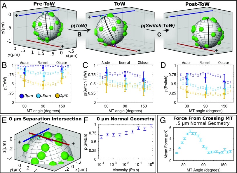
Fig. 3.

Mathematical model of navigational outcomes. (A) Snapshots of simulated cargo activity at an intersection (color coding as in Fig. 1B). Examples of Pre-ToW (A, Left), ToW (A, Center), and post-ToW (A, Right) states are shown. Motors bound to the primary MT are shown in cyan. Motors bound to the crossing MT are shown in magenta. Unbound motors are shown as green spherical protrusions from the cargo; sphere radius represents motor’s maximal reach. Bead’s prime meridian is demarcated to emphasize rotational movement. (B) Simulated probabilities to engage in ToW. Probability of undergoing ToW for each geometry is shown as thin symbols (error bars: SEM). Experimental data (Table 1) are shown as large symbols (error bars: 95% C.I.). Experimental data points for 0.5-μm geometries are shifted slightly horizontally to aid the eye. (C) Simulated probability to switch, given the cargo engaged in ToW. Simulated and experimental data (Table 2) represented as in B. (D) Simulated probability to switch, overall, i.e., the product of probability to ToW (B) and probability to switch, given ToW (C). Simulated and experimental data (Fig. 1B) are represented as in B. (E) Snapshot of a ToW for 0 μm, 90° geometry. Here, primary MT motors are blocked from passing the intersection by the crossing MT at 0 μm. Bound and unbound motors represented as in A. (F) Probability to switch increases with increasing simulated fluid viscosity. Error bars: SEM. Curve represents a linear fit. (G) Force exerted by crossing MT on the cargo for 0.5-μm geometries (mean ± SEM).