Fig. 1.

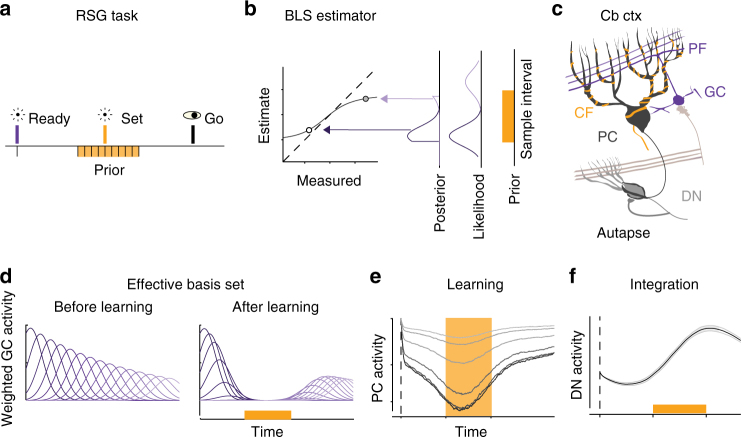
Task, cerebellar anatomy and the TRACE model. a Ready-Set-Go task. On each trial, participants measure a sample interval demarcated by two visual flashes– Ready (purple bar) and Set (orange bar) – and aim to reproduce that interval  immediately after Set (Go). The sample interval is drawn from a uniform prior distribution (orange distribution). b The Bayes-Least-Squares (BLS) estimator. A Bayesian observer computes the posterior based on the product of the prior and the likelihood function, and uses the mean of the posterior to estimate the interval. The plot shows the behavior of BLS for two measurements. The light and dark bell-shaped curves represent the likelihood function associated with those measurements. The BLS estimate is the expected value of the posterior, which is biased toward the mean of the prior (arrows) and away from the unity line (dashed). Due to scalar variability, the likelihood is wider for longer measurements (lighter likelihood function), resulting in a larger bias. c Schematic drawing of the relevant part of the cerebellar circuit. In the cerebellar cortex (Cb ctx), a Purkinje cell (PC, black) receives inputs from granule cells (GC, purple) via parallel fibers (PF), and from climbing fibers (CF, orange). PCs, in turn, project to and inhibit neurons in the dentate nucleus (DN), which additionally receive extra-cerebellar input (light brown) and autaptic (synapse onto self) input. d The effective basis set in TRACE, which reflects the GC basis set scaled by the GC to PC synaptic weights (i.e., Weighted GC activity). The plot shows weighted GC activity for a subset of GCs in the model. Left: Weighted GC activity before learning (sub-sampled). Right: Weighted GC activity after learning the prior. e PC activity profile based on TRACE simulations at different stages of  learning. The PC activity is shown after 10, 50, 100, 150, and 200 trials during learning (light to dark). f DN activity. The activity profile of DN reflects the integrated output of PCs, and is plotted after learning (trial 200). Shaded gray region indicates standard deviation. Traces in e and f do not correspond to any specific sample interval; instead, they show the expected response profiles in the absence of CF input (i.e., as if Set were never presented). Dashed lines in e and f correspond to the time of Ready, and the orange regions highlight the domain of the prior