
Figure 4.
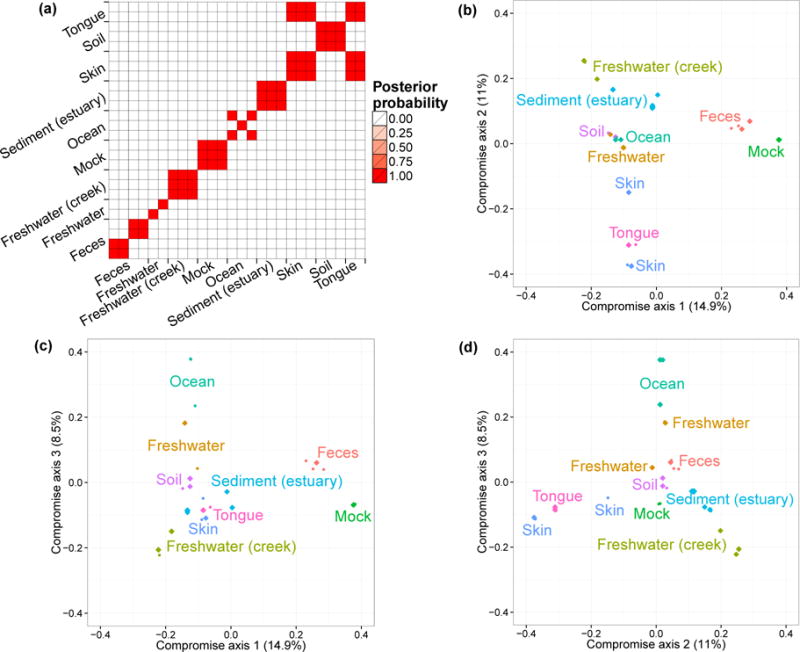
(a) Posterior Probability of each pair of biological samples (j, j′) being clustered together. The labels on axes indicate the environment of origin for each biological sample. (b–d) Ordination plots of biological samples and 95% posterior credible regions. We illustrate the first three compromise axes with three panels. Panel (b) plots projections on the first and second axes. Panel (c) plots projections on the first and third axes. Panel (d) plots projections on the second and third axes. The percentages on the three axes are the ratios of the corresponding S0 eigenvalues and the trace of the matrix. The credible regions for some biological samples are so small that appears as single points. Colors and annotated text indicate the environments.