Figure 2.

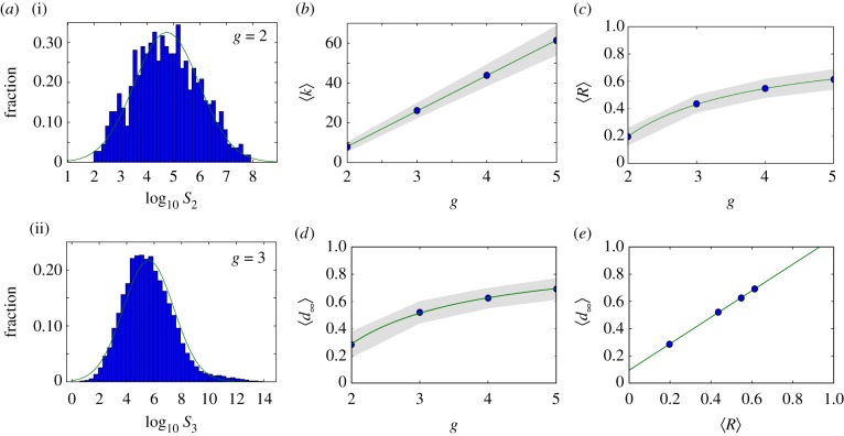
Neutral networks in toyLIFE. (a) The distribution of the number of genotypes per phenotype—phenotype abundance, S—for g = 2 (S₂, a(i)) follows a log-normal distribution, with probability density function , where μ is the mean and σ is the standard deviation of the normally distributed logarithm of the variable. Here μ = 4.742 and σ = 1.224, obtained using maximum-likelihood. For g = 3, the distribution of phenotype abundances (S₃, a(ii)) is again very close to a log-normal distribution with μ = 5.604 and σ = 1.838. The log-normal fit is worse than in (a) because there is a small bump in the right part of the distribution, where more abundant phenotypes are—due to the over representation of two-gene phenotypes (see text). (b) Average degree of nodes (circles) in neutral networks (see electronic supplementary material, figure S12 for the degree distribution) versus gene number g. The average degree 〈k〉 of a node grows linearly with gene number g, as 〈k〉 = − 27.6 + 17.8 g (line). (c) Average robustness (circles) versus gene number g. Robustness grows with gene number, and we can find a nonlinear relationship between both variables: 〈R〉 = 0.895 − 1.392/g (line). (d) There is a nonlinear relationship between g and 〈d_∞〉, the final distance that is reached in a random walk in which genotypes are forced to get away from the starting genotype every step: 〈d_∞〉 = 0.965 − 1.354/g (line). The circles represent 〈d_∞〉. (e) There is a linear relationship between 〈d_∞〉 and the average robustness of the genotypes as obtained in c, given by: 〈d_∞〉 = 0.094 + 0.972〈R〉 (line), very close to the 〈d_∞〉 = 〈R〉 fit. In all cases, the grey area encompasses two standard deviations, and the fits in (b–e) were obtained using the least-squares method. (Online version in colour.)