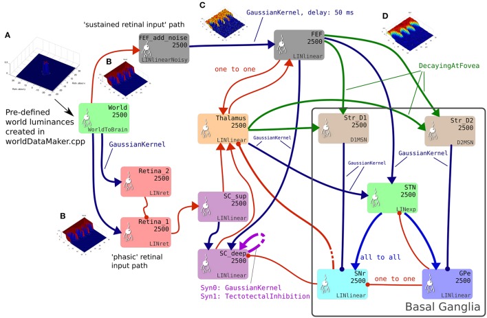
Figure 2.

The brain model. This is the SpineCreator “network layer” view of the model. Each box represents a neural population with 2,500 elements, arranged in a 50 × 50 grid. The SpineML component name is printed on the bottom right corner of each population box and the population name is at the top. The overall connectivity between populations is represented by the projection arrows with the color indicating the connectivity scheme (one-to-one connections are red, Gaussian kernel connections are dark blue and so on). Excitatory connections have arrowheads and inhibitory connections have circles, although for full details of the behavior of the connections, the weight-update and post-synapse component associated with each connection must be referred to. Briefly, the model comprises a World population, into which a retinotopically organized view of the world is introduced. This information is passed into cortical populations (FEF) and subcortical populations (SC) via a simple model of the retina. These feed a cortico-thalamo-basal ganglia loop, which selects which region of the deep layer of superior colliculus should be disinhibited, allowing activity to build up therein. The five populations comprising the basal ganglia are enclosed in a gray outline. Note that substantia nigra pars compacta is not modeled here, instead the level of dopamine in the striatum is set via a parameter in the Str_D1 and Str_D2 populations. (A) Fixation cross input in Cartesian eye frame. (B) Fixation cross input in retinotopic co-ordinates. (C) Fixation cross with noise added. (D) After blurring, input is passed to BG populations.