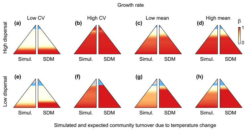
Figure 3.

Temporal community turnover along an elevational temperature gradient (β-diversity, represented by the gradient from white to red, see legend in panel d) following climate warming. The left section of the mountains represents the results of simulations (“Simul.”), while the right section represents the expected turnover obtained by simply stacking species distribution model projections (“SDM”). Shown are eight scenarios that differ depending on dispersal ability (rows) and growth rate within the species pool (a, e: coefficient of variation [CV] = 0.1; b, f: CV = 1/√3; c, g: mean = 0.2; d, h: mean = 0.5; a-d: d = 10^-1; e-h: d = 10^-4). In each panel, all other parameters except the ones specified in the header of their line and column were set to the average value of their respective distribution (see Table S1). The lowest elevation communities are not displayed (see Appendix S1). Communities at the highest elevations resulting from colonization of previously unoccupied habitat are coloured in blue, while communities that remain empty despite warming are in light grey. Note that outcomes of temporal community turnover obtained from stacking SDM projections can also differ slightly among panels due to different initial conditions (i.e. initial burn-in period that allowed the meta-communities to equilibrate).