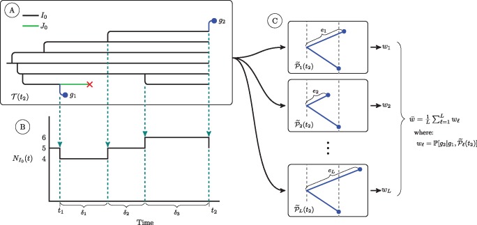
Fig. 10.

A schematic of quantities used in calculation of the conditional density of a diagnosis and the conditional probability of a genetic sequence. At (A) we show a simulated transmission tree. For simplicity, this tree only has individuals of class I₀ and class J₀. Dashed arrows fall from events in the transmission tree that change the count of I₀ individuals in the population. At (B) we show a plot of the trajectory of the I₀ class. This plot shows the quantities we use to calculate the cumulative hazard of diagnosis for the I₀ class, ${\Lambda }_0$, over an interval of time from t₁ to t₂. We first subdivide the time interval into R subintervals over which the number of I₀ individuals is constant (indicated with dashed lines). We let the number of I₀ individuals in the rth subinterval be $N_{I_0,r}$. The cumulative hazard of diagnosis is then: ${\Lambda }_0={\rho }_0{\sum }_{r=1}^R{\delta }_r{N}_{I_0,r}$. The cumulative hazards of diagnosis for the other two classes of undiagnosed individuals are computed in the same fashion. At (C) we show the set of L subtrees of the phylogeny that we use to numerically estimate the conditional probability of sequence g₂ under our relaxed clock model. The $\ell \text{th}$ subtree is constructed by augmenting $\tilde{\mathcal{P}}(t_1)$ with a new edge with length $e_{\ell }$ drawn from a Gamma distribution parameterized as described in the text. For each of these L subtrees we use the peeling algorithm to compute $w_{\ell }=\mathbb{P}[g_2|g_1,{\tilde{\mathcal{P}}}_{\ell }(t_2)]$, the conditional probability of observing sequence g₂ given sequence g₁ and the structure of ${\tilde{\mathcal{P}}}_{\ell }(t_2)$. The average of these conditional probabilities is a numerical estimate of the conditional probability of g₂ under our relaxed clock model. For simplicity, here we do not show the case in which the edge length of g₂ splits an existing edge; this case requires a beta bridge to apportion the length of the split edge so as to maintain Gamma distributed edge lengths. For this more complicated case, see figure 9.