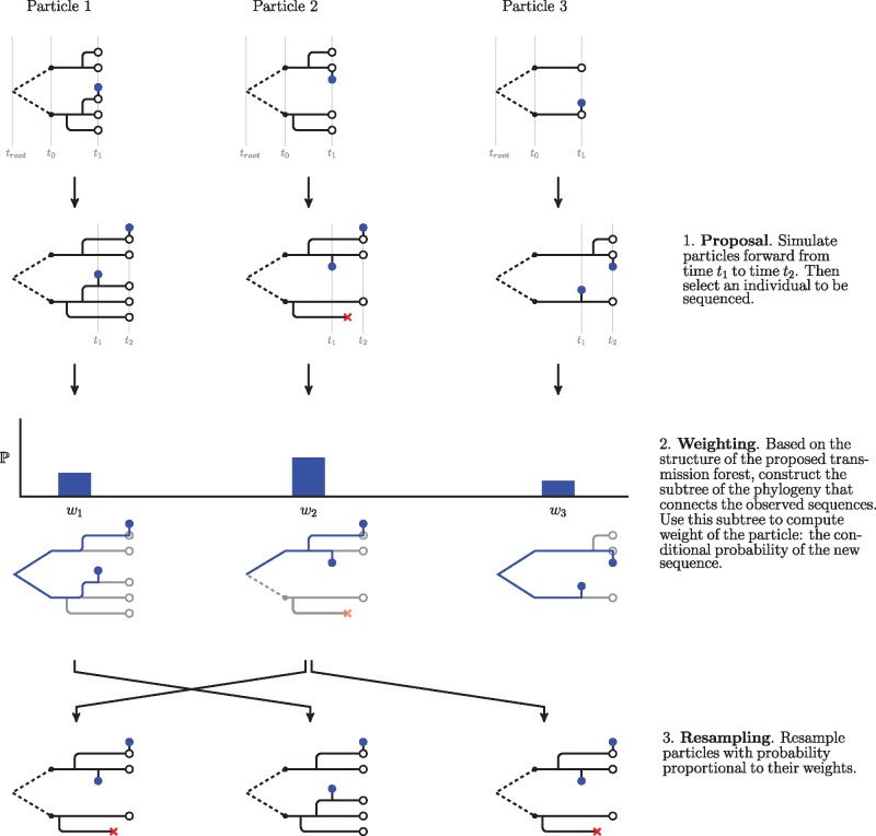
Fig. 7.

A schematic of the particle filter. Here, we show steps to run the filter from the first sequence to the second. Transmission forests are shown in black and phylogenies that connect observed sequences, $\tilde{\mathcal{P}}(t)$, are shown in blue. Observed sequences are depicted as blue dots. This schematic shows how the algorithm uses just-in-time construction of state variables to ease computational costs. Although the model describes how $\mathcal{P}(t)$ relates to $\mathcal{T}(t)$ across all branches of the transmission tree, the algorithm only constructs the subtree of the phylogeny needed to connect the observations (and therefore evaluate conditional probabilities of sequences). Note that in our implementation of the particle filter we introduce additional procedures in the proposal and weighting steps. These procedures, which are detailed below, allow for more accurate assessment of a particle’s weight (through hierarchical sampling) and estimation of the conditional probability of a sequence under a relaxed clock. In our current implementation (supplementary algorithm S1, Supplementary Material online), assimilation of each data point is followed by systematic resampling (Arulampalam et al. 2002; Douc et al. 2005); future developments may aim to increase efficiency further using alternative resampling schemes.