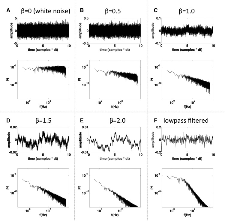
Figure 1.
Illustration of white noise and different flavors of pink noise. A–E, Noise with different 1/f exponents (β, where spectral power scales as 1fβ in log-log coordinates). The upper axis of each panel shows the time series and the lower axis shows the power spectrum; β specifies the slope of the power spectrum in units of log power versus log frequency, so if β = 0, then the noise is white (flat power spectrum, roughly equal power in all frequencies, each sample independent of all other samples). Notice that as β increases, the time series becomes more and more dominated by low-frequency fluctuations, as indicated by the slope of the spectra. Time series are shown for values of β between 0 and 2 to illustrate the way that time series change qualitatively as β changes. F, Same noise series as in A after lowpass filtering with a first-order Butterworth filter (cutoff frequency of 1 Hz).

