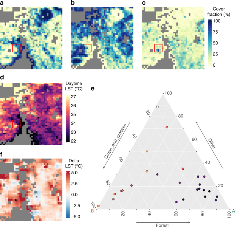
Fig. 7.

Illustration of the methodology for retrieving the local biophysical signal associated to potential vegetation change. The input consists of vegetation cover fraction maps for different classes, in this case: forests (a), crops/grasses (b) and other (c); and the spatial variation of the target biophysical variable, here day-time land surface temperature (LST) (d). e Ternary diagram showing the values of the 25 pixels in the red boxes of a–c respectively plotted in the three axes. The colour of the points represents the corresponding values of the biophysical variable. The regression in the compositional space allows the estimation of LST at the vertices of the triangle: vertex A representing a full forest cover and vertex B representing 100% cover of crops/grasses. The difference between these values is the estimated change in LST following a total change from forests to crops/grasses for the pixel in the centre of the 5 by 5 window. f The estimated change in LST for the transition from forests to crops/grasses for the entire region. Grey areas are masked out because of the topographical filtering or lack of co-occurrence of either forests or crops/grasses. The size of the pixels is 0.05° or ~5.5 km at the equator