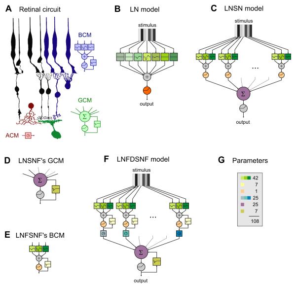
Figure 1. A progression of circuit models constrained by retinal anatomy.
(A) Schematic of the circuit upstream of a ganglion cell in the vertebrate retina. Photoreceptors (P) transduce the visual stimulus into electrical signals that propagate through bipolar cells (B) to the ganglion cell (G). At both synaptic stages one finds both convergence and divergence, as well as lateral signal flow carried by horizontal (H) and amacrine (A) cells. The bipolar cell and its upstream circuitry is modeled by a spatio-temporal filter, a nonlinearity and feedback (bipolar cell module, BCM; blue). The amacrine cell introduces a delay in lateral propagation (amacrine cell module, ACM; red). The ganglion cell was modeled by a weighted summation, another nonlinearity, and a second feedback function (ganglion cell module, GCM; green). Drawings after Polyak, 1941.
(b) LN model. A different temporal filter is applied to the history of each bar in the stimulus. The outputs of all these filters are summed over space. The resulting signal is passed through an instantaneous nonlinearity.
(c) LNSN model. The stimulus is first processed by partially overlapping, identical BCMs, each of which consists of its own spatio-temporal filter and nonlinearity. Their outputs are weighted and summed by the GCM, which then applies another instantaneous nonlinearity to give the model’s output. For display purpose the BCMs are shown here to span only 3 stimulus bars, but they spanned 7 bars in the computations.
(d) LNSNF model. This is identical to the previous one, except that the GCM (depicted here) has an additional feedback loop around its nonlinearity.
(e) LNFSNF model. This is identical to the previous one, except that the BCMs (one of which is depicted here) have an additional feedback loop around their nonlinearities. This new feedback function is the same for all BCMs.
(f) LNFDSNF model. This is identical to the previous one, except that there is a delay inserted between each BCM and the GCM. These delays are allowed to vary independently for each BCM.
(g) A count of the free parameters in the LNFDSNF model, color coded as in the model diagram. Except for the total (108), the numbers here also apply to the LNSN, LNSNF, and LNFSNF models. The LN model has 186 free parameters in the linear filter (31 spatial positions, each with 6-parameter temporal filter as in Error! Reference source not found.–Error! Reference source not found.) and 1 in the nonlinearity. See also Figures S1 and S3.

