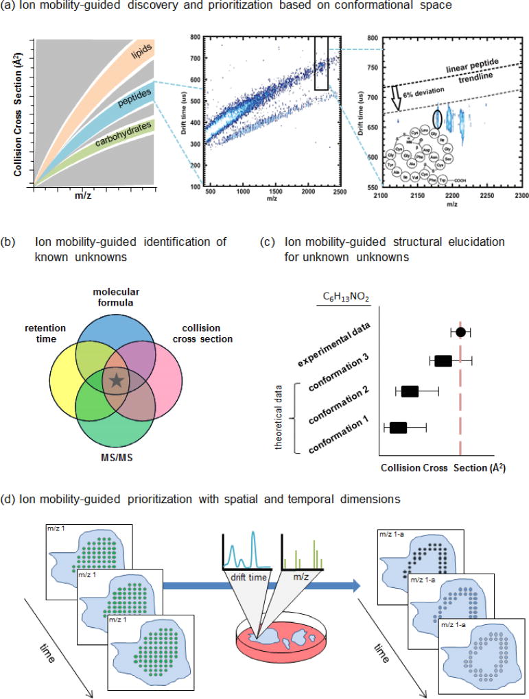
Figure 1.

Applications of metabolomic workflows utilizing ion mobility-mass spectrometry for discovery of secondary metabolite natural products. (a) (Left) IM-MS mobility-mass correlation plots reveal trends of various molecular classes within conformational space. (Middle) Deviations of species from predicted trendlines can be exploited for secondary metabolite prioritization. (Right) This region annotates a peak with dense gas-phase packing efficiency that falls nearly 12% below the linear peptide trendline for this m/z. This compound was identified as siamycin II, a tricyclic peptide, and confirmed by isolation and NMR analyses. Reproduced with permission from [17]. Copyright 2012 American Chemical Society. (b) The Venn diagram represents candidate identifications based on individual data dimensions. Mass spectrometry yields accurate mass and isotope pattern information that can be used to determine molecular formula, liquid chromatography yields retention time, and ion mobility yields drift time/CCS. The goal of including multiple descriptors is to filter candidate space and remove false positives, ultimately leading to a true positive identification (represented here by a star). (c) Computational methods can be used to simulate 3-D structural conformations and calculate theoretical CCS values for comparison with experimental data. Conformations that are consistent with the experimental CCS range are prioritized for structural elucidation. In this mock example, three conformations were predicted for an unknown species with a molecular formula of C₆H₁₃NO₂. Their theoretical CCS values were compared with the experimental CCS value, revealing conformation 3 as a plausible structure. (d) MSI experiments generate m/z spectra for each spatial coordinate. The integration of an ion mobility dimension enables isobaric species to be separated resulting in more accurate ion images. In this example, m/z 1 appears with uniform signal (green dots) across a sample. Mobility data revealed an isobar, m/z 1-a, with signal (blue dots) that appears as a border around the sample. Further temporal data would enable tracking of this spatial data as a function of time.