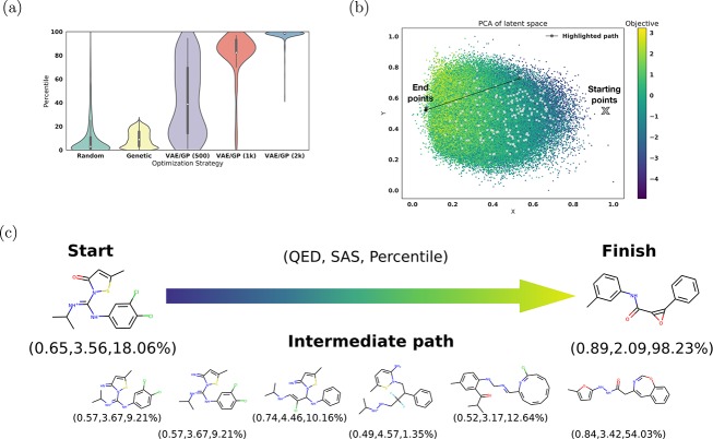
Figure 4.

Optimization results for the jointly trained autoencoder using 5 × QED – SAS as the objective function. (a) shows a violin plot which compares the distribution of sampled molecules from normal random sampling, SMILES optimization via a common chemical transformation with a genetic algorithm, and from optimization on the trained Gaussian process model with varying amounts of training points. To offset differences in computational cost between the random search and the optimization on the Gaussian process model, the results of 400 iterations of random search were compared against the results of 200 iterations of optimization. This graph shows the combined results of four sets of trials. (b) shows the starting and ending points of several optimization runs on a PCA plot of latent space colored by the objective function. Highlighted in black is the path illustrated in part (c). (c) shows a spherical interpolation between the actual start and finish molecules using a constant step size. The QED, SAS, and percentile score are reported for each molecule.