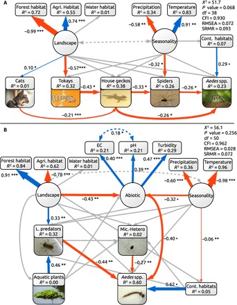
Fig. 1. Path diagrams for the terrestrial and aquatic SEMs.

The terrestrial model (n = 70) used a robust maximum likelihood estimator (A). In the aquatic model (n = 156), turbidity (clear/murky), aquatic plants (presence/absence), and Aedes spp. larvae (presence/absence, due to zero inflation) were modeled as binomial variables, using a weighted least squares estimation with robust standard errors (B). R² values represent variance explained. Model fit was assessed using χ² statistics, comparative fit index (CFI), root mean square errors of approximation (RMSEA), and standardized root mean square residual (SMRS). Solid arrows display paths from independent to dependent variables, dotted arrows display covariances, circles are latent variables, and rectangles are measured variables. Blue arrows, positive effects; red arrows, negative effects; gray arrows, nonsignificant effects. Effects represent correlations based on the best fitting covariance structure for each model and might be causative, but are not so by definition. Path coefficients (standardized effect sizes) are near each arrow. ***P < 0.001, **P < 0.01, *P < 0.05, and ^•P < 0.1. “Agri. habitat,” “Water habitat,” and “Forest habitat” are total area of agricultural, surface water, and forested areas in the landscape, which was a 250-m-radius area centered on the focal building. “Precipitation” represents the total monthly precipitation, and “Temperature” represents the monthly (aquatic model) and two-monthly (terrestrial model) mean temperature before sampling. “Cont. habitats” represents the number of container-like habitats in the landscape. EC is electrical conductivity, and pH is the acidity of container habitat water. L. predators, large predators; Mic.-Hetero, micro-Heteroptera.