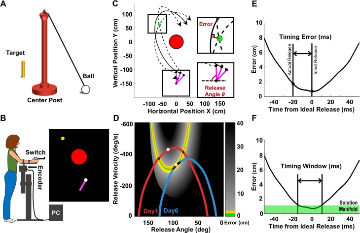
Fig 1. Model throwing task, experimental set-up and analyses of timing measures.

(A) Real skittles task. (B) Experimental setup of the virtual throwing task; manipulandum and screen display. (C) Top down view of skittles workspace. Red circle is the post, green circle is target and pink bar represents the lever arm. The ball trajectory shown by the solid line incurred a non-zero error; the two dashed ball trajectories were successful throws hitting the target. The two insets illustrate the definition of the error around the target (top) and the release angle (below). (D) Execution space of the skittles task is spanned by two execution variables, release angle and velocity. Assuming each point in the space is a ball release, the error is calculated and shown in color code: green denotes the solution manifold, where each point leads to a hit below the error threshold of 1.1cm. The adjacent yellow band is the error threshold, denoting throws that hit the target but with an error larger than 1.1cm and smaller than 2.5cm (no intersection of ball trajectory with target). Two representative arm trajectories of the same subject are plotted in execution space, red from Day 1, blue from Day 6; white dots represent ball releases. The release on the red trajectory resulted in a large error; the release on the blue trajectory in a successful hit. (E) Each arm trajectory can be represented as an “error trajectory”, assuming each point on the trajectory is a ball release associated with an error. The timing error was calculated as the difference between the time of actual and ideal release. (F) Using the same “error trajectory” the timing window was quantified as the time that the trajectory would yield errors below the success threshold of 1.1cm, i.e. within the solution manifold.