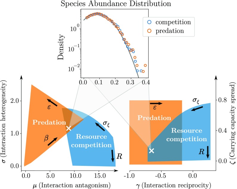
Fig. 3.

Different models visit the generic parameter space $(\mu ,\sigma ,\gamma ,\zeta )$ defined in Eq. 3 as we vary their model-specific control parameters (bold arrows, defined in Materials and Methods). We illustrate, in the $(\mu ,\sigma )$ and $(\gamma ,\zeta )$ planes, the regions visited by two models. In orange is predation with mean intensity $\beta \in [0.1,25]$ and conversion efficiency $\epsilon \in [\mathrm{0,1}]$ (in this model, $\zeta$ is a free parameter). In blue is resource competition with resources number $R\in [{10}^2,{10}^4]$ and consumption heterogeneity ${\sigma }_{\xi }\in [0.1,0.6]$. (Inset) An example where a competitive community and a predator–prey community display identical species abundance distributions, well predicted by the theory (solid line), corresponding to the parameter values marked by the cross. We explain, in Discussion and in SI Appendix, Reference Model and Community Properties, under which conditions these distributions are predicted to be narrow (e.g., normal) or fat-tailed (e.g., lognormal); see also refs. 11 and 23.