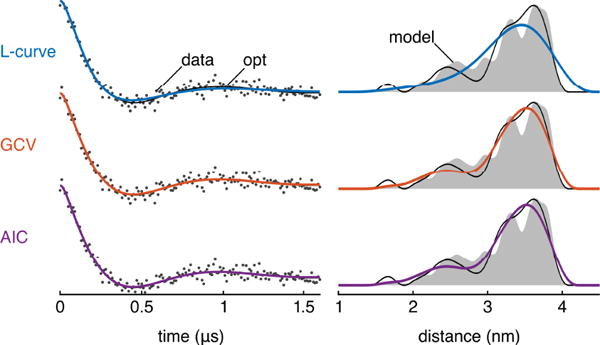
Figure 7.

Example case comparing the LR2u L-curve, GCV, and AIC methods (dataset 115333). For this particular test case, each method features an inefficiency very close to that method’s overall median inefficiency (LR2u 1.38, GCV 1.09, AIC 1.09). Left column: the simulated data are shown as grey dots, the Tikhonov fit with optimum α is shown as a black line, and the Tikhonov fits for LR2u, GCV, and AIC are shown as blue, orange, and purple lines, respectively. Right column: the model P is shown in grey, the Tikhonov solution for P with optimum α is shown as a black line, and the Tikhonov Ps for LR2u, GCV, and AIC are shown as blue, orange, and purple lines, respectively. In all cases, the L2 operator was used.
