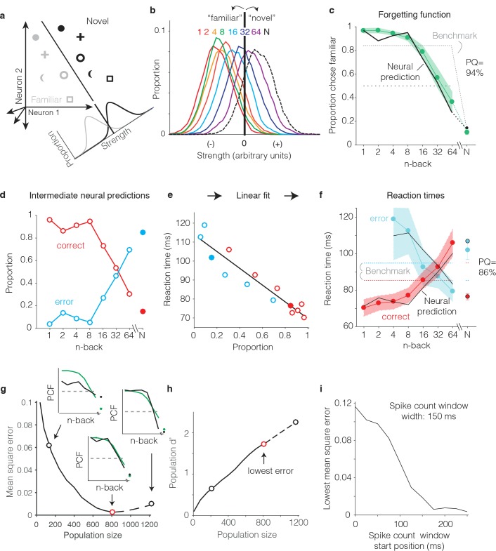
Figure 6. Transforming IT neural data into behavioral predictions.

In all panels, behavioral and neural data correspond to the data pooled across the two monkeys and methods are illustrated through application of only one linear decoder (the FLD). (a) A cartoon depiction of how memory strength was measured for each n-back. Shown are the hypothetical population responses of 2 neurons to different images (represented by different shapes) shown as novel (black) versus as familiar (gray). The line depicts a linear decoder decision boundary optimized to classify images as novel versus as familiar. Distributions across images within each class are calculated by computing the linearly weighted sum of each neuron’s responses and subtracting a criterion. (b) Distributions of the linearly weighted IT population response, as a measure of memory strength, shown for novel images (black dotted) and familiar images parsed by n-back (rainbow), for a population of 799 units. To compute these distributions, a linear decoder was trained to parse novel versus familiar across all n-back via an iterative resampling procedure (see Materials and methods). (c) Black: the neural prediction of the behavioral forgetting function, computed as the fraction of each distribution in panel b that fell on the ‘familiar’ (i.e. left) side of the criterion. Behavioral data are plotted with the same conventions as Figure 3a,c. Prediction quality (PQ) was measured relative to a step function benchmark (gray dotted) with matched average performance (see text). (d) The first step in the procedure for estimating reaction times, shown as a plot of the proportions of each distribution from panel b predicted to be correct versus wrong, as a function of n-back. Solid and open circles correspond to novel and familiar trials, respectively. Note that the red curve (correct trials) simply replots the predictions from panel c and the blue curve (error trials) simply depicts those same values, subtracted from 1. (e) A plot of the proportions plotted in panel d versus the monkeys’ mean reaction times for each condition, and a line fit to that data. (f) The final neural predictions for reaction times, computed by passing the data in panel d through the linear fit depicted in panel e. Behavioral data are plotted with the same conventions as Figure 3b,d. Also shown are the benchmarks used to compute PQ (labeled), computed by passing the benchmark values showing in panel c through the same process. (g) Mean squared error between the neural predictions of the forgetting function and the actual behavioral data, plotted as a function of population size. Solid lines correspond to the analysis applied to recorded data; the dashed line corresponds to the analysis applied to simulated extensions of the actual data (see Figure 6—figure supplement 1). Insets indicate examples of the alignment of the forgetting function and FLD neural prediction at three different population sizes, where green corresponds to the actual behavioral forgetting function and black corresponds to the neural prediction. PCF = proportion chose familiar. The red dot indicates the population size with the lowest error (n = 799 units). (h) Overall population d’ for the novel versus familiar task pooled across all n-back, plotted as a function of population size with the highlighted points from panel g indicated. (i) The analysis presented in panel g was repeated for spike count windows 150 ms wide shifted at different positions relative to stimulus onset. Shown is the minimal MSE for each window position. All other panels correspond to spikes counted 150–400 ms.

Figure 6—figure supplement 1. Extrapolating SCC and FLD predictions to larger sized populations.

To extrapolate neural predictions beyond the population sizes that we had recorded, we modeled the population response distributions at each n-back (Figure 6b) as Gaussian, and we estimated the means and standard deviations of each distribution at different population sizes by extending the trajectories computed from our data (solid lines) to estimates at larger population sizes (dotted lines). (a) In the case of the SCC, the mean population response was computed as the grand mean spike count across the population, and consequently did not grow with population size. We thus extended these trajectories with a simple linear fit to the values computed from the data. Shown are the population means computed for the novel images (black), the familiar images parsed by n-back (cyan) and the mean that corresponds to the criterion placement (red). In contrast, the standard deviations of these trajectories decreased as a function of population size and to extend these trajectories, we fit a two-parameter function (see Materials and methods). (b) In the case of the FLD, the population mean was computed as a weighted sum and grew linearly with population size. We extended these trajectories with a simple linear fit to the values computed from the data. In contrast, the FLD population standard deviation trajectories grew in a nonlinear manner, and to extend these trajectories, we fit a two-parameter function (see Materials and methods).